GTSAM Posts

Introduction

In our previous post we discussed some basic concepts to solve linear and nonlinear factor graphs and to extract uncertainty estimates from them. We reviewed that the Fisher information matrix corresponds to an approximation of the inverse covariance of the solution, and that in the nonlinear case, both the solution and its covariance estimate are valid for the current linearization point only.

While the nonlinear case effectively allows us to model a bunch of problems, we need to admit we were not too honest when we said that it was everything we needed to model real problems. Our formulation so far assumed that the variables in our factor graph are vectors, which is not the case for robotics and computer vision at least.

This second part will review the concept of manifold and how the reference frames affect the formulation of our factor graph. The tools we cover here will be also useful to define probability distributions in a more general way, as well as to extend our estimation framework to more general problems.

Getting non-Euclidean

In robotics we do not estimate the state of a robot only by their position but also its orientation. Then we say that is its pose, i.e position and orientation together, what matters to define its state.

Representing pose is a tricky thing. We could say “ok, but let’s just append the orientation to the position vector and do everything as before” but that does not work in practice. Problem arises when we want to compose two poses $\mathbf{T}_1 = (x_1, y_1, \theta_1)$ and $\mathbf{T}_2 = (x_2, y_2, \theta_2)$. Under the vector assumption, we can write the following expression as the composition of two poses:

\[\begin{equation} \mathbf{T}_1 + \mathbf{T}_2 = \begin{bmatrix} x_1\\ y_1 \\ \theta_1 \end{bmatrix} + \begin{bmatrix} x_2 \\ y_2 \\ \theta_2\end{bmatrix} = \begin{bmatrix} x_1 + x_2 \\ y_1+y_2 \\ \theta_1 + \theta_2\end{bmatrix} \end{equation}\]

This is basically saying that it does not matter if we start in pose $\mathbf{T}_1$ or $\mathbf{T}_2$, we will end up at the same final pose by composing both, because in vector spaces we can commute the elements. But this does not work in reality, because rotations and translations do not commute. A simple example is that if you are currently sitting at your desk, and you stand up, rotate 180 degrees and walk a step forward, is completely different to stand up, walk a step forward and then rotate 180 degrees (apart from the fact that you will hit your desk if you do the latter).

So we need a different representation for poses that allow us to describe accurately what we observe in reality. Long story short, we rather have to represent planar poses as $3\times3$ matrices known as rigid-body transformations:

\[\begin{equation} \mathbf{T}_1 = \left[\begin{matrix} \cos{\theta_1} && -\sin{\theta_1} && x_1 \\ \sin{\theta_1} && \cos{\theta_1} && y_1 \\ 0 && 0 && 1\end{matrix} \right] = \left[\begin{matrix} \mathbf{R}_1 && \mathbf{t}_1 \\ 0 && 1\end{matrix}\right] \end{equation}\]

Here $\mathbf{R}_1 = \left[ \begin{matrix} \cos{\theta_1} && -\sin{\theta_1}\\ \sin{\theta_1} && \cos{\theta_1}\end{matrix} \right]$ is a 2D rotation matrix, while $\mathbf{t}_1 = \left[ \begin{matrix}x_1 \ y_1 \end{matrix}\right]$ is a translation vector. While we are using a $3\times3$ matrix now to represent the pose, its degrees of freedom are still $3$, since it is a function of $(x_1, y_1, \theta_1)$.

Working with transformation matrices is great, because we can now describe the behavior we previously explained with words using matrix operations. If we start in pose $\mathbf{T}_1$ and we apply the transformation $\mathbf{T}_2$:

\[\begin{equation} \mathbf{T}_1 \mathbf{T}_2 = \left[\begin{matrix} \mathbf{R}_1 && \mathbf{t}_1 \\ 0 && 1\end{matrix}\right] \left[\begin{matrix} \mathbf{R}_2 && \mathbf{t}_2 \\ 0 && 1\end{matrix}\right] = \left[\begin{matrix} \mathbf{R}_1 \mathbf{R}_2 && \mathbf{R}_1 \mathbf{t}_2 + \mathbf{t}_1 \\ 0 && 1\end{matrix}\right] \end{equation}\]

We can now rewrite the same problem as before but now using our transformation matrices:

\begin{equation} \mathbf{T}_{i+1} = \mathbf{T}_i \ \Delta\mathbf{T}_i \end{equation}

Here we are saying that the next state $\mathbf{T}_{i+1}$ is gonna be the previous state $\mathbf{T}_{i}$ plus some increment $\Delta\mathbf{T}_i$ given by a sensor -odometry in this case. Please note that since we are now working with transformation matrices, $\Delta\mathbf{T}_i$ is almost everything we need to model the problem more accurately, since it will represent a change in both position and orientation.

Now, there are two things here that we must discuss before moving on, which are fundamental to make everything consistent. We will review them carefully now.

The importance of reference frames

While some people (myself included) prefer to write the process as we did before, applying the increment on the right-hand side:

\[\begin{equation} \mathbf{T}_{i+1} = \mathbf{T}_i \ \Delta\mathbf{T}_i \end{equation}\]

Others do it in a different way, on the left-hand side:

\[\begin{equation} \mathbf{T}_{i+1} = \Delta\mathbf{T}_i \ \mathbf{T}_i \end{equation}\]

These expressions are not equivalent as we already discussed because rigid-body transformations do not commute. However, both make sense under specific conventions. We will be more explicit now by introducing the concept of reference frames in our notation. We will use the notation presented by Paul Furgale in his blog post “Representing Robot Pose: The good, the bad, and the ugly”.

Let us say that the robot trajectory in space is expressed in a fixed frame; we will called it the world frame $W$. The robot itself defines a coordinate frame in its body, the body frame $B$.

Then we can define the pose of the robot body $B$ expressed in the world frame $W$ by using the following notation:

\[\begin{equation} \mathbf{T}_{WB} \end{equation}\]

Analogously, using we can express the pose of the origin/world $W$ expressed in the robot frame $B$:

\[\begin{equation} \mathbf{T}_{BW} \end{equation}\]

According to this formulation, the first is a description from a fixed, world frame while the left-hand one does it from the robot’s perspective. The interesting thing is that we can always go from one to the other by inverting the matrices:

\[\begin{equation} \mathbf{T}_{WB}^{-1} = \mathbf{T}_{BW} \end{equation}\]

So the inverse swaps the subindices, effectively changing our point-of-view to describe the world.

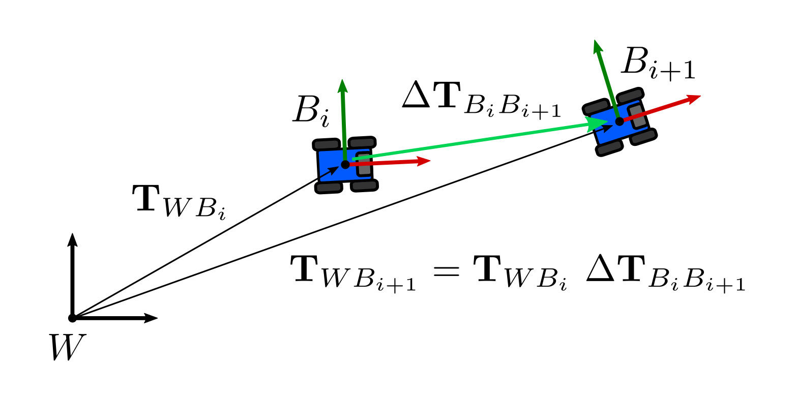
Using one or the other does not matter. The important thing is to stay consistent. In fact, by making the frames explicit in our convention we can always check if we are making mistakes. Let us say we are using the first definition, and our odometer is providing increments relative to the previous body state. Our increments $\Delta\mathbf{T}_i$ will be $\Delta\mathbf{T}_{B_{i} B_{i+1} }$, i.e, it is a transformation that describes the pose of the body at time $i+1$ expressed in the previous one $i$.

Hence, the actual pose of the body at time $i+1$ expressed in the world frame $W$ is given by matrix multiplication of the increment on the right side:

\[\begin{equation} \mathbf{T}_{WB_{i+1}} = \mathbf{T}_{WB_i} \ \Delta\mathbf{T}_{B_{i} B_{i+1} } \end{equation}\]

We know this is correct because the inner indices cancel each other, effectively representing the pose at $i+1$ in the frame we want:

\[\begin{equation} \mathbf{T}_{WB_{i+1}} = \mathbf{T}_{W {\bcancel{B_i}} } \ \Delta\mathbf{T}_{ {\bcancel{B_{i}}} B_{i+1} } \end{equation}\]

Since we applied the increment from the right-hand side, we will refer to this as the right-hand convention.

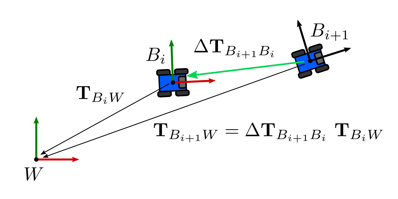
If we want to apply the increment to $\mathbf{T}_{BW}$, we would need to invert the measurement:

\[\begin{equation} \Delta\mathbf{T}_{B_{i+1} B_{i}} = \Delta\mathbf{T}_{B_{i} B_{i+1}}^{-1} \end{equation}\]

so we can apply the transformation on the left-hand side:

\[\begin{equation} \mathbf{T}_{B_{i+1}W} = \Delta\mathbf{T}_{B_{i+1} B_{i}} \mathbf{T}_{B_i W} \end{equation}\]

which we will refer onward as left-hand convention.

In GTSAM we use the right-hand convention: we assume that the variables are expressed with respect to a fixed frame $W$, hence the increments are applied on the right-hand side.

It is important to have this in mind because all the operations that are implemented follow this. As a matter of fact, 3D computer vision has generally used left-hand convention because it is straightforward to apply the projection models from the left:

\[\begin{equation} {_I}\mathbf{p} = \mathbf{K}_{IC}\ \mathbf{T}_{CW}\ {_{W}}\mathbf{P} \end{equation}\]

Here we made explicit all the frames involved in the transformations we usually can find in textbooks: An homogeneous point ${_{W}}\mathbf{P}$ expressed in the world frame $W$, is transformed by the extrinsic calibration matrix $\mathbf{T}_{CW}$ (a rigid body transformation ) which represents the world $W$ in the camera frame $C$, producing a vector ${_{C}}\mathbf{P}$ in the camera frame (not shown). This is projected onto the image by means of the intrinsic calibration matrix $\mathbf{K}_{IC}$, producing the vector $_I\mathbf{p}$, expressed in the image frame $I$.

Since in GTSAM the extrinsic calibration is defined the other way to be consistent with the right-hand convention, i.e $\mathbf{T}_{WC}$, the implementation of the CalibratedCamera handles it by properly inverting the matrix before doing the projection as we would expect:

\[\begin{equation} {_I}\mathbf{p} = \mathbf{K}_{IC}\ (\mathbf{T}_{WC})^{-1}\ {_{W}}\mathbf{P} \end{equation}\]

They are not simply matrices

The second important point we need to discuss, is that while rigid-body transformations are nice, the new expression we have to represent the process presents some challenges when trying to use it in our factor graph using our previous method:

\[\begin{equation} \mathbf{T}_{WB_{i+1}} = \mathbf{T}_{WB_i} \ \Delta\mathbf{T}_{B_{i} B_{i+1} } \end{equation}\]

In first place, we need to figure out a way to include the noise term $\eta_i$ we used before to handle the uncertainties about our measurement $\Delta\mathbf{T}_{B_{i} B_{i+1} }$, which was also the trick we used to generate the Gaussian factors we use in our factor graph. For now, we will say that the noise will be given by a matrix $\mathbf{N}_i \in \mathbb{R}^{4\times4}$, which holds the following:

\[\begin{equation} \mathbf{T}_{WB_{i+1}} = \mathbf{T}_{WB_i} \ \Delta\mathbf{T}_{B_{i} B_{i+1}} \mathbf{N}_i \end{equation}\]

Secondly, assuming the noise $\mathbf{N}_i$ was defined somehow, we can isolate it as we did before. However, we need to use matrix operations now:

\[\begin{equation} \mathbf{N}_i = (\mathbf{T}_{WB_i} \ \Delta\mathbf{T}_{B_{i} B_{i+1}})^{-1} \mathbf{T}_{WB_{i+1}} \end{equation}\]

and we can manipulate it a bit for clarity:

\[\begin{equation} \mathbf{N}_i = (\Delta\mathbf{T}_{B_{i} B_{i+1}})^{-1} (\mathbf{T}_{WB_i})^{-1} \mathbf{T}_{WB_{i+1}} \end{equation}\]

If we do the subindex cancelation trick we did before, properly swapping the indices due to the inverses, we can confirm that the error is defined in frame $B_{i+1}$ and expressed in frame $B_{i+1}$. This may seen counterintuitive, but in fact describes what we want: the degree of mismatch between our models and measurements to express the pose at frame $B_{i+1}$, which ideally should be zero.

However, the error is still a matrix, which is impossible to include as a factor in the framework we have built so far. We cannot compute a vector residual as we did before, nor we are completely sure that the matrix $\mathbf{N}_i$ follows some sort of Gaussian distribution.

We need to define some important concepts used in GTSAM to get a better understanding on how the objects are manipulated.

Some objects are groups

First of all, some objects used in GTSAM are groups. Rigid-body transformations Pose3 and Pose2 in GTSAM), rotation matrices (Rot2 and Rot3) and quaternions, and of course vector spaces (Point2 and Point3) have some basic operations that allow us to manipulate them. These concepts have been discussed in previous posts at the implementation level:

Composition: How to compose 2 objects from the same manifold, with associativity properties. It is similar to the addition operation for vectors.
Identity: An identity operator under the composition/between.
Inverse: An element that when composed with its inverse becomes the identity.

The previous 3 operations allows us to define the operation between, which computes the difference between 2 objects from the same group, similarly to a subtraction operation.

Since the operations can be defined in different ways for each kind of object (it is different to compose rotation matrices than quaternions or vectors for instance), some authors define special operators to refer to composition/between operations. Some examples are the box-plus $\boxplus$ for composition and box-minus $\boxminus$ for between as done by Hertzberg et al., Blanco-Claraco, Bloesch et al., and the Kindr library.

However, composition can be defined from the left or the right side because composition is associative but is not distributive. This is the same problem we described before when talking about reference frames and how to add small increments with the left and right hand conventions, since both are valid depending on our decisions or other authors’. While we can be clear about our own decisions, it is important to be aware of the definitions of each author because sometimes are not clearly stated. Solà et al for example make the difference explicit by defining left-$\oplus$ and right-$\oplus$ for composition using left-hand convention or right-hand convention respectively, but we need to be careful to recognize each other’s choices.

We recall again that in GTSAM and the rest of this post we use the right convention (pun intended), because we represent our poses with respect to a fixed world frame $W$ and the increments are defined with respect to the body frame $B$.

Some are manifolds

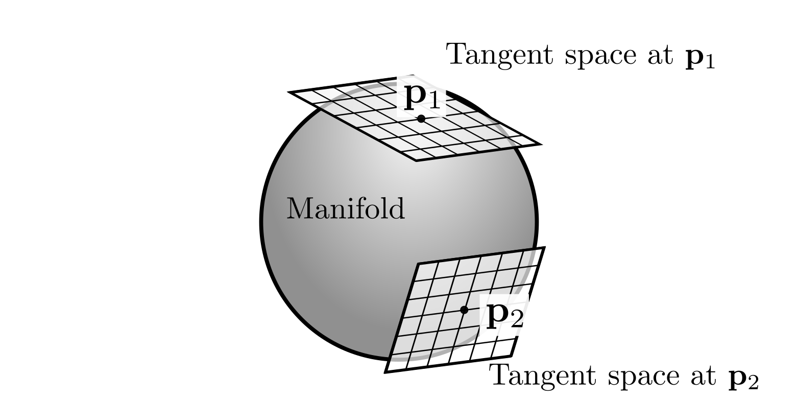
Additionally, rigid-body transformations, rotation matrices, quaternions and even vectors are differentiable manifolds. This means that even though they do not behave as Euclidean spaces at a global scale, they can be locally approximated as such by using local vector spaces called tangent spaces. The main advantage of analyzing all these objects from the manifold perspective is that we can build general algorithms based on common principles that apply to all of them.

Manifold and tangents spaces — While a manifold have a non-Euclidean structure, it can be locally approximated by tangent spaces. In the figure, we illustrate different tangent spaces defined at the objects $\mathbf{p}_1$ and $\mathbf{p}_2$ on the manifold.

As we briefly mentioned before, objects such as rotation matrices are difficult to manipulate in the estimation framework because they are matrices. A 3D rotation matrix $\mathbf{R}$ represents 3 orientations with respect to a reference frame but, in raw terms, they are using 9 values to do so, which seems to overparametrize the object. However, the constraints that define a rotation matrix -and consequently the manifold- such as orthonormality $\mathbf{R}^{T}\mathbf{R} = \mathbf{I}$ and $\text{det}(\mathbf{R}) = 1$ make the inherent dimensionality of the rotation still 3. Interestingly, this is exactly the dimensionality of the tangent spaces that can be defined over the manifold.

That is what makes working with manifolds so convenient: All the constraints that are part of the definition of the object are naturally handled, and we can work in tangent vector spaces using their inherent dimension. The same happens for rigid-body transformations (6 dimensions represented by a 16 elements matrix), quaternions (3 orientations represented by a 4D vector), and even objects that are not groups, such as unit vectors.

In order to work with manifolds, we need to define 2 operations, which are the key to transform objects between them and the tangent spaces:

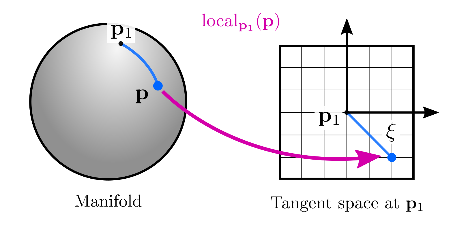
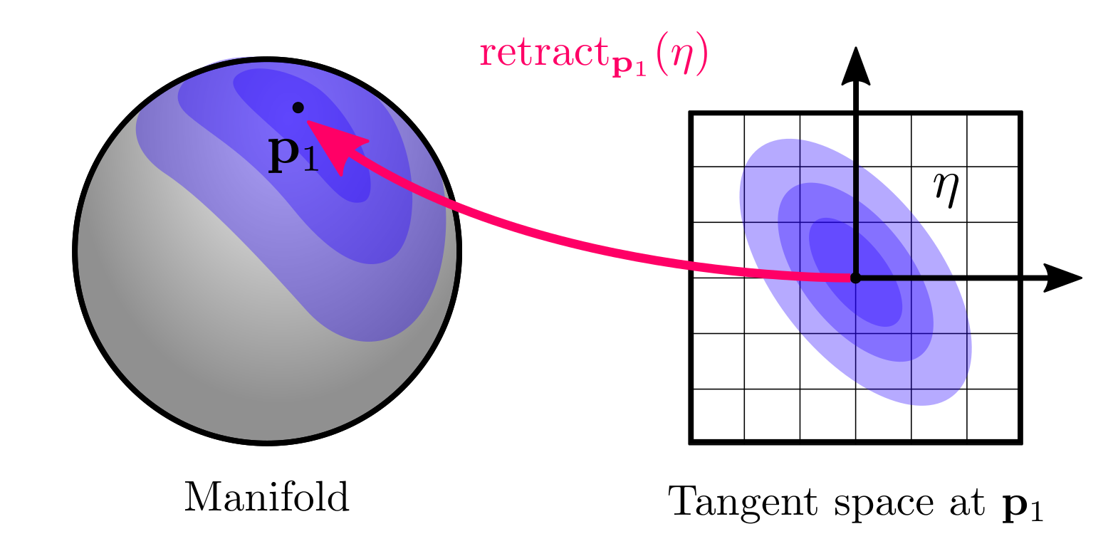
Retract or retraction: An operation that maps elements $\mathbf{\xi}$ from the tangent space at $\mathbf{p}_1$ to the manifold: $\mathbf{p} = \text{retract}_{\mathbf{p}_1}(\mathbf{\xi})$.
Local: the opposite operation: mapping elements $\mathbf{p}$ from the manifold to the tangent space $\mathbf{\xi} = \text{local}_{\mathbf{p}_1}(\mathbf{p})$

Retract operation on a manifold — The *retract* operation maps an element $\mathbf{\xi}$ defined in the tangent space at $\mathbf{p}_1$ back to the manifold.

Retract operation on a manifold simplified — An alternative figure to represent the retraction that will be used in the rest of the post, since it shows the interactions between the manifold and the tangent space more explicitly. We can clearly observe that the element $\mathbf{p}$ generated by the retraction is also defined with respect to $\mathbf{p}_1$ on the manifold.

Local operation on a manifold — The *local* operation does the opposite, and maps an element $\mathbf{p}$ defined with respect to $\mathbf{p}_1$ as an vector $\mathbf{\xi}$ in the tangent space.

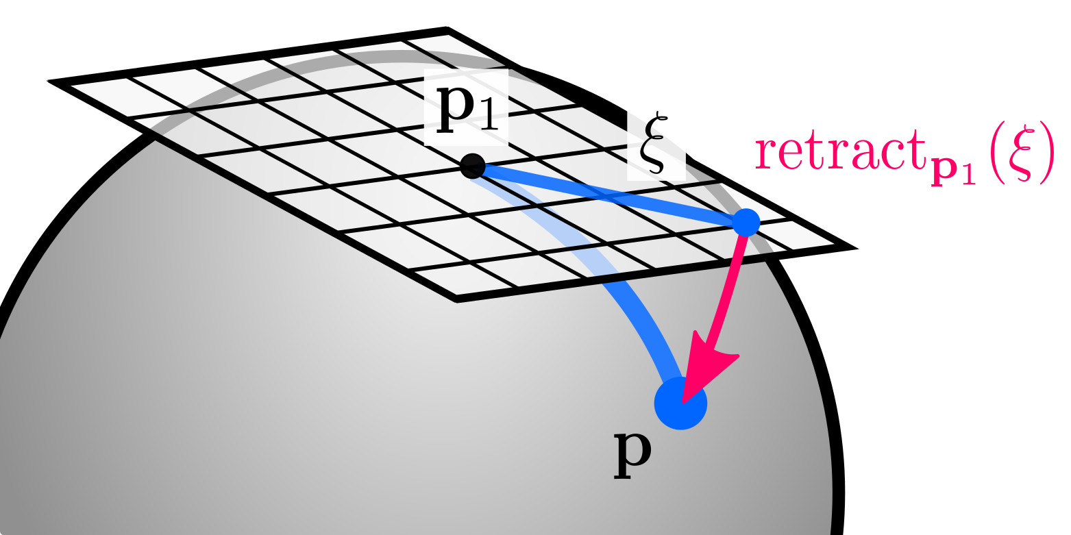
Retractions are the fundamental concept to solve optimization problems and to define uncertainties on manifolds. While the former will be covered later in this post with an example, it is useful to explain the latter now. The general idea is that we can define distributions on the tangent space, and map them back on the manifold using the retraction. For instance, we can define a zero-mean Gaussian variable $\eta \sim Gaussian(\mathbf{0}_{n\times1}, \Sigma)$ in the tangent space centered at $\mathbf{p}$ and use the retraction:

\[\begin{equation} Gaussian(\mathbf{p}_1, \mathbf{\eta}) := \text{retract}_{\mathbf{p}_1}(\mathbf{\eta}) \end{equation}\]

which graphically corresponds to:

Gaussian on a manifold — Using the retraction, we can define Gaussians on the tangent space centered at some element $\mathbf{p}_1$ and map them back on the manifold to construct Gaussians on the manifold with mean $\mathbf{p}_1$ and covariance $\text{Cov}(\eta) = \Sigma$.

Please note that we have defined the retraction from the right, since this matches the convention used by GTSAM, which coincidently also matches the composition operator for groups. However, in the literature we can find different definitions: Barfoot and Furgale (2014, left-hand convention), Forster et al (2017, right-hand convention), and Mangelson et al. (2020, left-hand convention) are some examples. Other definitions to define probability distributions on manifolds include Calinon (2020) and Lee et al. (2008), please refer to their work for further details.

And others are both: Lie groups

In GTSAM we only need the objects to be differentiable manifolds in order to optimize them in the estimation framework, being groups is not a requirement at all. However, it is important to be aware that some of the objects we deal with are both groups and differentiable manifolds, known as Lie groups, which is the formulation generally found in state estimation literature.

Lie groups are both groups and differentiable manifolds. They define a tangent space at the identity that allows to represent any object on the manifold through a retraction defined at the identity, known as exponential map, as well as a local operation also at the identity - the logarithm map.

Objects such as rigid-body matrices and quaternions are Lie groups. 2D rigid-body transformations are elements of the Special Euclidean group $\text{SE(2)}$, while 2D and 3D rotations are from the Special Orthogonal groups $\text{SO(2)}$ and $\text{SO(3)}$ respectively. 3D rigid-body transformations are objects of $\text{SE(3)}$ and we can use those definitions to define the operations we described before for groups and manifolds:

Composition: Matrix multiplication $\mathbf{T}_{1} \ \mathbf{T}_{2}$.
Identity: Identity matrix $\mathbf{I}$.
Inverse: Matrix inverse $(\mathbf{T}_{1})^{-1}$
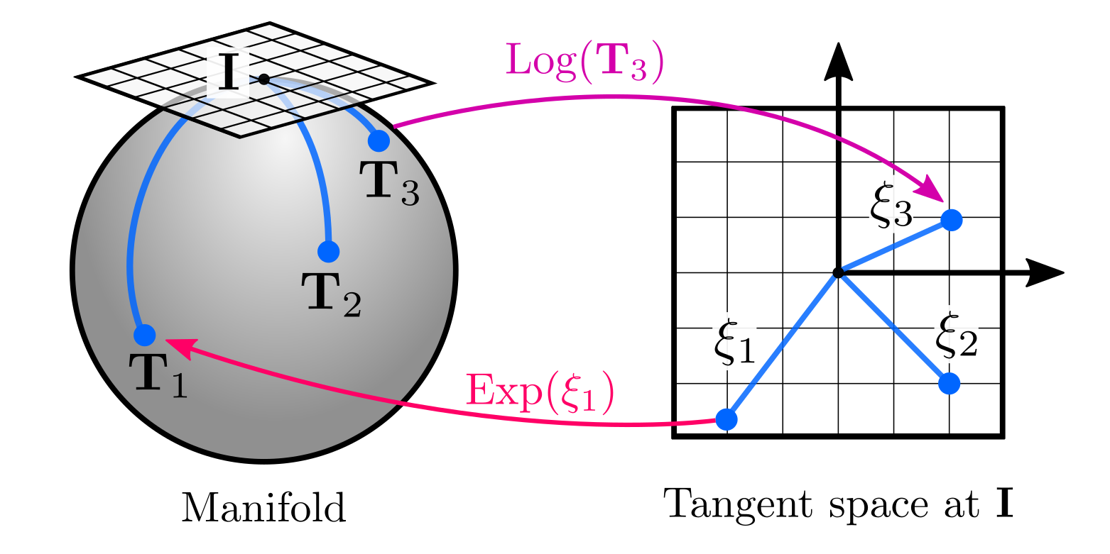
Retract: The retraction is defined at the tangent space at the identity, which is known as the exponential map of $\text{SE(3)}$: $\text{retract}_{\mathbf{I}}(\mathbf{\xi}) := \text{Exp}(\mathbf{\xi})$.
Local: It is also defined at the identity and known as the logarithm map of $\text{SE(3)}$: $\text{local}_{\mathbf{I}} := \text{Log}(\mathbf{T}_{1} )$.

Please note here that we used capitalized $\text{Log}(\cdot) := \text{log}( \cdot)^{\vee}$ and $\text{Exp}(\cdot):=\text{exp}( (\cdot)^{\wedge})$ operators for simplicity as used by Forster et al (2017), and Solà et al. (2020), since they are easy to understand under the retractions perspective. Refer to Solà et al. for a more detailed description, including the relationship between tangents spaces and the Lie algebra.

In GTSAM, 3D poses are implemented as Pose3 objects and we can think of them as $\text{SE(3)}$ elements. Therefore, to keep things simple, we will stay using the logarithm map and exponential map to talk about their retraction and local operators. However, GTSAM also allows us to use alternative retractions for some cases, which would be like using other Lie groups to represent poses, such as the $\mathbb{R}^{3}\times\text{SO}(3)$ group, which is explained here.

Reference frames on manifolds

Reference frames are preserved when applying the local and retract operations. We will cover a few important ideas using $\text{SE(3)}$, since it is related to our original problem of pose estimation.

First of all, when we talked about the tangent space defined at the identity, in physical terms it refers to having a fixed, global frame, which we use to express our poses. Then, when using the local operation defined as the logarithm map of $\text{SE(3)}$, we obtain a vector $_W\mathbf{\xi}_{W} \in \mathbb{R}^{6}$ (sometimes also called tangent vector or twist), which is defined in the tangent space at the world frame:

\[\begin{equation} {_W}\mathbf{\xi} = \text{Log}(\mathbf{T}_{WB_i} ) \end{equation}\]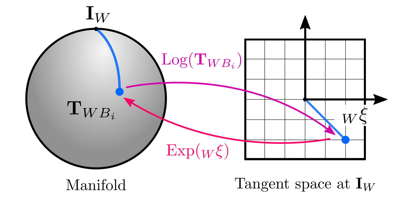

In this example, the tangent space at the identity represents the world frame, on which any transformation $\mathbf{T}_{WB_i}$ expressed in the world frame can be defined.

Additionally, we can add incremental changes to a transformation using the retraction, which for $\text{SE(3)}$ is done with the exponential map as follows:

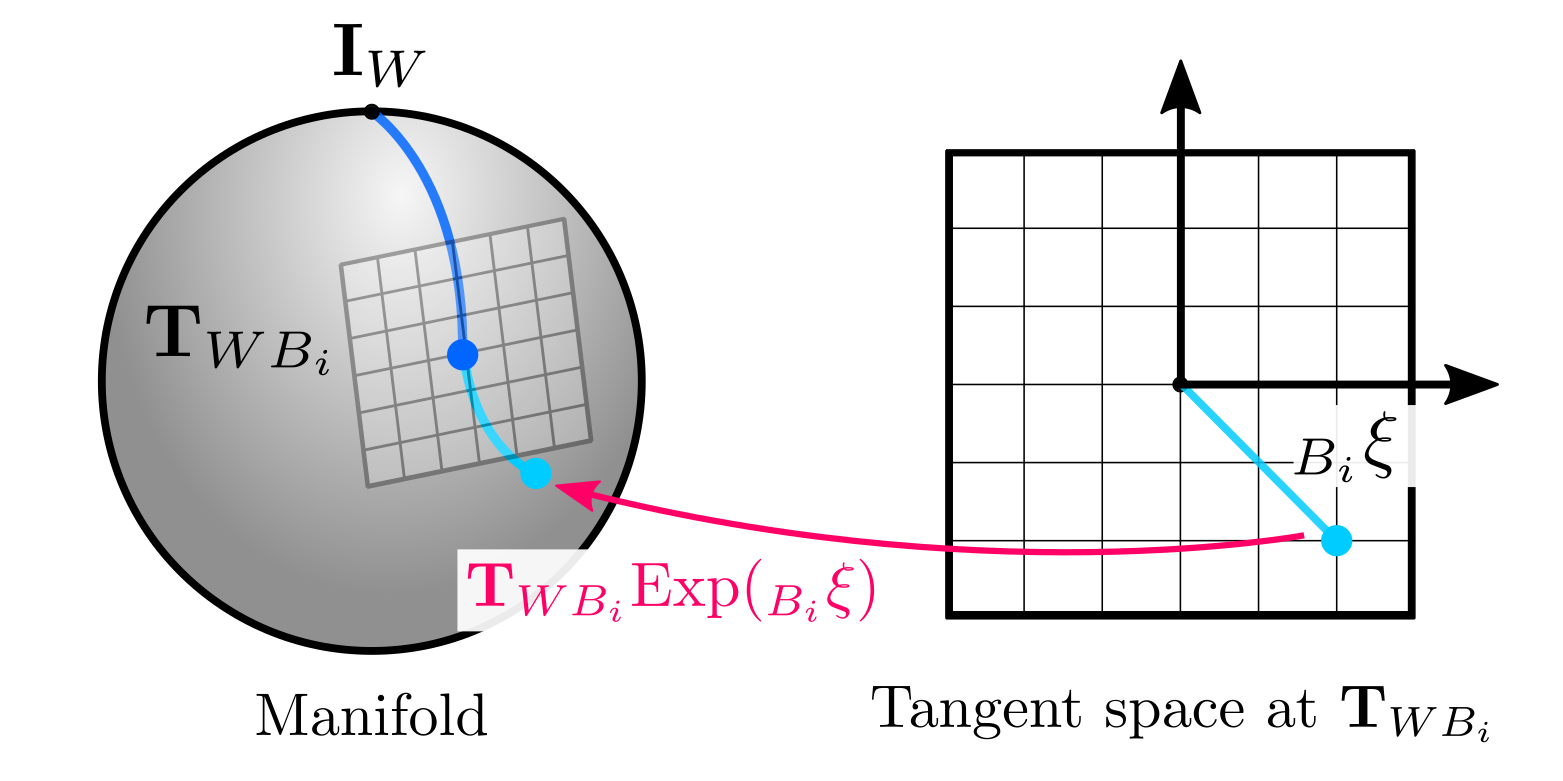
\[\begin{equation} \mathbf{T}_{WB_{i+1}} = \mathbf{T}_{WB_i} \text{Exp}( {_{B_i}}\mathbf{\xi}) \end{equation}\]

In this case we added an increment from the body frame at time $i$, that represents the new pose at time $i+1$. Please note that the increments are defined with respect to a reference frame, but they do not require to specify the resulting frame. Their meaning (representing a new pose at time $i+1$) is something that we -as users- define but is not explicit in the formulation. (While we could do it, it can lead to confusions because in this specific case we are representing the pose at the next instant but we can also use retractions to describe corrections to the world frame as we will see in the final post.)

The graphical interpretation with the manifold is consistent with our general definition of retractions and frames. Using the exponential map on the right is defining a tangent space at $\mathbf{T}_{WB_i}$, which can be interpreted as a new reference frame at $B_i$, which we used to define the increment:

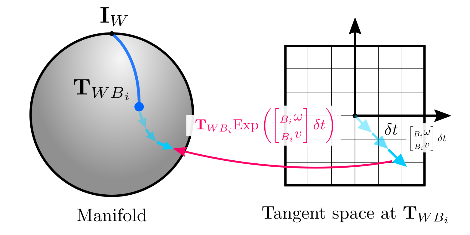
Retraction with frames — When we add a small increment ${_{B_i}}\mathbf{\xi}$ to the pose $\mathbf{T}_{WB_i}$, the expression $\mathbf{T}_{WB_i} \text{Exp}( {_{B_i}}\mathbf{\xi})$ corresponds to the retraction defined for the tangent space at $\mathbf{T}_{WB_i}$.

The incremental formulation via retractions is also convenient when we have local (body frame) velocity measurements -also known as twists- $({_{B_i}}\omega, {_{B_i}}{v})$, with ${_{B_i}}\omega \in \mathbb{R}^{3}, {_{B_i}}v \in \mathbb{R}^{3}$ and we want to do dead reckoning:

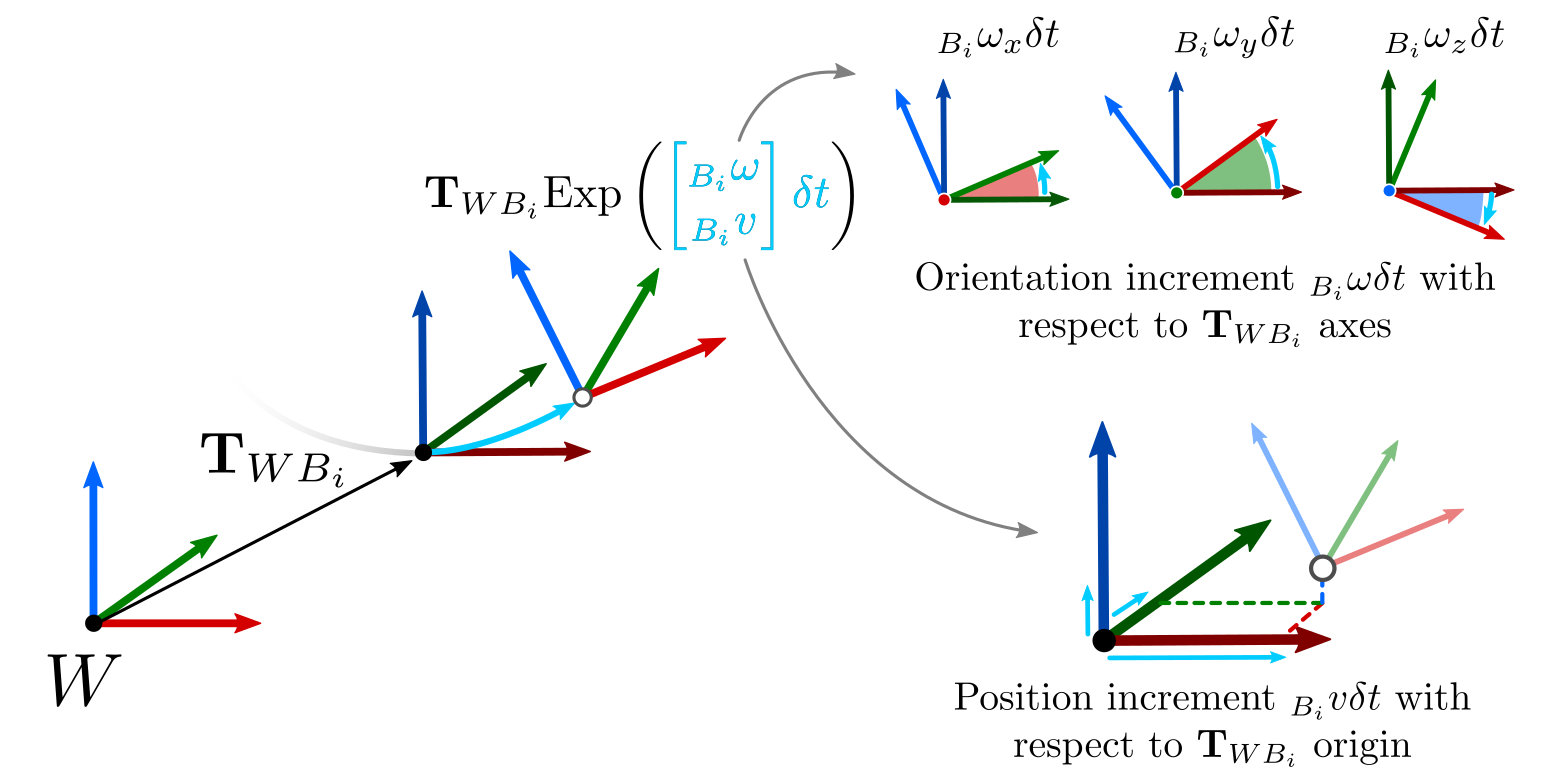
\[\begin{equation} \mathbf{T}_{WB_{i+1}} = {\mathbf{T}_{WB_i}} \text{Exp}\left( \begin{bmatrix} _{B_i}\omega \\ _{B_i} v \end{bmatrix}\ \delta t \right) \end{equation}\]

The product $\begin{bmatrix} _{B_i}\omega \ \delta t \\ _{B_i} v \ \delta t\end{bmatrix}$ represents the tangent vector resulting from time-integrating the velocity, which is map onto the manifold by means of the $\text{SE(3)}$ retraction:

Retraction with velocities — The same formulation can be used to map velocities into increments via retractions/exponential map. In this case, the time increment $\delta t$ controls the length of the curve that is projected on the manifold when we do dead-reckoning.

This last example is also useful to understand the physical meaning of the retraction/local operations in the case of 3D poses, which is not always clear. An interesting aspect of illustrating this with $\text{SE}(3)$ is that the meaning also applies if we use rotations only ($\text{SO}(3)$, $\text{SO}(2)$) or 2D poses ($\text{SE}(2)$):

Retraction with velocities, physical interpretation — This figure illustrates the physical meaning of the $\text{SE}(3)$ retraction of the dead-reckoning example. In light blue we show the increment applied to pose ${\mathbf{T}_{WB_i}}$, which generates a *new* frame. At the right hand side we illustrate the decomposed increment: orientation at the top, and position at the bottom. Each component of the *orientation increment* represents a change with respect to each rotation axis defined by the body pose at ${\mathbf{T}_{WB_i}}$ (rotations with respect to $X$, $Y$ and $Z$ axes, respectively, are shown). When combined, the vector represents an *axis-angle* representation of the rotation increment. *Position increments* (right-side, bottom) are easier to interpret because they only represent a shift in position with respect to ${\mathbf{T}_{WB_i}}$'s origin. Since the retraction actually *combines* both orientation and position increments on the manifold, it generates a smooth trajectory as shown on the left-hand side (light blue).

Some remarks on the retract and local operations

Lastly, we would like to share some important remarks that are not always stated in the math but can become real issues during the implementation. First, we need to be careful about the convention of the order of the components in the retraction/local operation (yes, more conventions again). Having clarity about the definition that every software or paper uses for these operations, even implicitly, is fundamental to make sense of the quantities we put into our estimation problems and the estimates we extract.

For instance, the definition of the $\text{SE(3)}$ retraction we presented, which matches Pose3 in GTSAM, uses an orientation-then-translation convention, i.e, the 6D tangent vector has orientation in the first three coordinates, and translation in the last three $\mathbf{\xi} = (\phi, \rho)$, where $\phi \in \mathbb{R}^3$ denotes the orientation components while $\rho \in \mathbb{R}^3$ the translational ones. On the other hand, Pose2 uses translation-then-orientation $(x, y, \theta)$ for historical reasons.

This is also ties the definition of the covariances. For Pose3 objects, for instance, we must define covariance matrices that match the definition and meaning of the tangent vectors. In fact, the upper-left block must encode orientation covariances, i.e, our degree of uncertainty for each rotation axis, while the bottom-right encodes position covariances:

\[\begin{equation} \left[\begin{matrix} \Sigma_{\phi\phi} & \Sigma_{\phi\rho} \\ \Sigma_{\phi\rho}^{T} & \Sigma_{\rho\rho} \end{matrix}\right] \end{equation}\]

This is of paramount importance because, for example, the previous covariance matrix does not match the convention used in ROS to store the covariances in PoseWithCovariance. Similar issues can arise when using different libraries or software, so we must be aware of their conventions. Our advice is to always check the retraction/exponential map definition if not stated in the documentation.

Bringing everything together

Now we can return to our original estimation problem using rigid-body transformations. Let us recall that we defined the following process model given by odometry measurements:

\[\begin{equation} \mathbf{T}_{WB_{i+1}} = \mathbf{T}_{WB_i} \ \Delta\mathbf{T}_{B_{i} B_{i+1}} \mathbf{N}_i \end{equation}\]

We reported two problems before:

We needed to define the noise $\mathbf{N}_i$ as a Gaussian noise, but it was a $4\times4$ matrix.
When isolating the noise to create the residual, we ended up with a matrix expression, not vector one as we needed in our estimation framework.

We can identify now that our poses are objects of $\text{SE(3)}$, hence we can use the tools we just defined.

Defining the noise

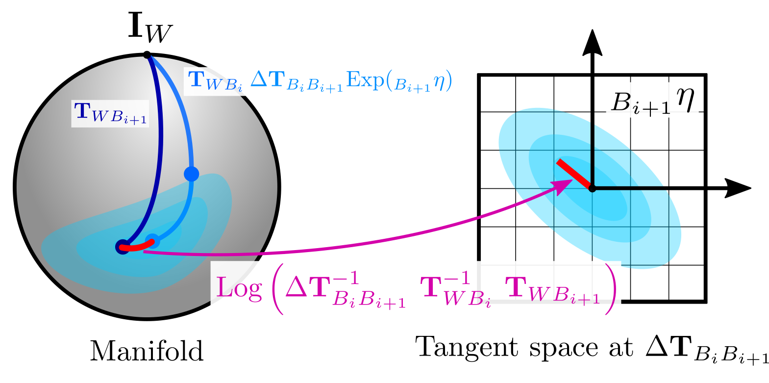
The first problem of defining the noise appropriately is solved by using probability distributions on manifolds as we described before. We define a zero-mean Gaussian in the tangent space at $\Delta\mathbf{T}_{B_{i} B_{i+1}}$ and retract it onto the manifold:

\[\begin{equation} \mathbf{T}_{WB_{i+1}} = \mathbf{T}_{WB_i} \ \Delta\mathbf{T}_{B_{i} B_{i+1}} \text{Exp}(_{B_{i+1}}\mathbf{\eta}) \end{equation}\]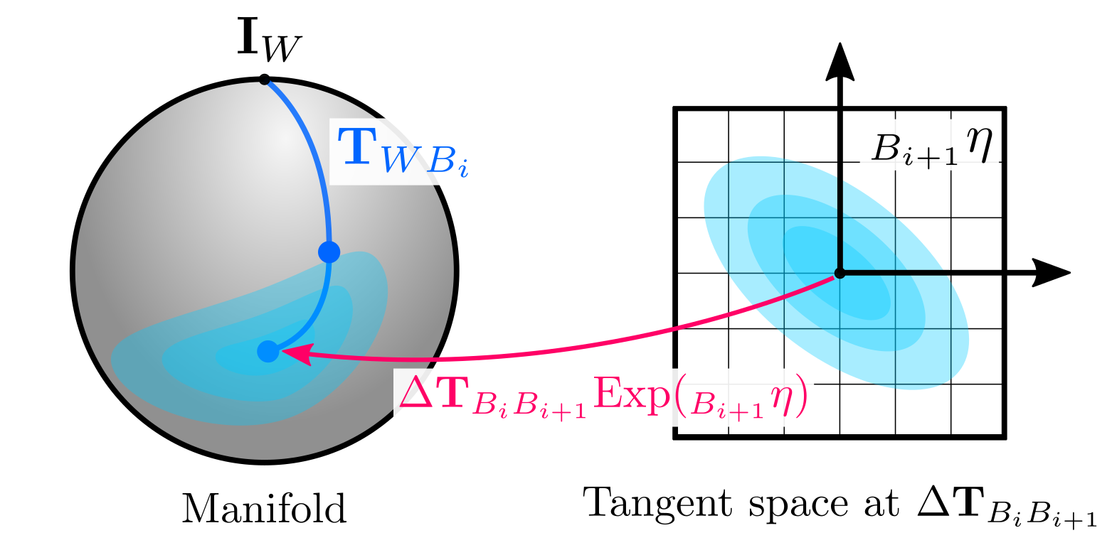

Defining noise for the relative increment. — Graphical interpretation of the definition of the noise, which is defined in frame $B_{i+1}$ and mapped using the retraction.

where we have defined ${_{B_{i+1}}}\eta \sim Gaussian(\mathbf{0}_{6\times1},\ _{B_{i+1}}\Sigma)$. Please note that in order to match our right-hand convention, the covariance we use must be defined in the body frame at time $i+1$, i.e $B_{i+1}$. Additionally, the covariance matrix must follow the same ordering defined by the retraction as we mentioned before.

Defining the residual

Having solved the first problem, we can now focus on the residual definition. We can isolate the noise as we did before, which holds:

\[\begin{equation} \text{Exp}( {_{B_{i+1}}}\mathbf{\eta}) = \Delta\mathbf{T}_{B_{i} B_{i+1}}^{-1}\ \mathbf{T}_{WB_i}^{-1} \ \mathbf{T}_{WB_{i+1}} \end{equation}\]

We can now apply the local operator of the manifold on both sides to map the residual to the tangent space (recall we are using the logarithm map for $\text{SE(3)}$ elements for simplicity):

\[\begin{equation} _{B_{i+1}}\mathbf{\eta} = \text{Log}\left( \Delta\mathbf{T}_{B_{i} B_{i+1}}^{-1}\ \mathbf{T}_{WB_i}^{-1} \ \mathbf{T}_{WB_{i+1}} \right) \end{equation}\]

Since the noise is defined in the tangent space, both sides denote vector expressions in $\mathbb{R}^{6}$. Both also correspond to zero-mean Gaussians, hence the right-hand side can be used as a proper factor in our estimation framework. In fact, the expression on the right side is exactly the same used in GTSAM to define the BetweenFactor.

We must also keep in mind here that by using the local operation, the residual vector will follow the same ordering. As we mentioned before for Pose3 objects, it will encode orientation error in the first 3 components, while translation error in the last ones. In this way, if we write the expanded expression for the Gaussian factor, we can notice that all the components are weighted accordingly by the inverse covariance as we reviewed before (orientation first, and then translation):

\[\begin{equation} \begin{split} \mathbf{r}_{\text{between}}(\mathbf{T}_{WB_i}, \mathbf{T}_{WB_{i+1}}) &= \left|\left| \text{Log}\left( \Delta\mathbf{T}_{B_{i} B_{i+1}}^{-1}\ \mathbf{T}_{WB_i}^{-1} \ \mathbf{T}_{WB_{i+1}} \right)\right|\right|^{2}_{\Sigma_i} \\ & = \text{Log}\left( \Delta\mathbf{T}_{B_{i} B_{i+1}}^{-1}\ \mathbf{T}_{WB_i}^{-1} \ \mathbf{T}_{WB_{i+1}} \right)^{T} \ \Sigma_i^{-1} \\ & \qquad \qquad \qquad \text{Log}\left( \Delta\mathbf{T}_{B_{i} B_{i+1}}^{-1}\ \mathbf{T}_{WB_i}^{-1} \ \mathbf{T}_{WB_{i+1}} \right) \end{split} \end{equation}\]

The factor is now a nonlinear vector expression that can be solved using the nonlinear optimization techniques we presented before. In fact, GTSAM already implements Jacobians for the local operator of all the objects implemented, which simplifies the process. However, there are subtle differences that we must clarify.

First, since the factor defines a residual in the tangent space at the current linearization point, the optimization itself is executed in the tangent space defined in the current linearization point. This means that when we linearize the factors and build the normal equations, the increment ${_{B_i}}\delta\mathbf{T}^{k}$ we compute lies in the tangent space.

For this reason, we need to update the variables on the manifold using the retraction. For example, for $\text{SE(3)}$:

\[\begin{equation} \mathbf{\tilde{T}}_{WB_i}^{k+1} = \mathbf{T}_{WB_i}^k \text{Exp}( {_{B_i}}\delta\mathbf{T}^{k} ) \end{equation}\]

The second important point, is that the covariance that we can recover from the information matrix, will be also defined in the tangent space around the linearization point, following the convention of the retraction. It means that if our information matrix at the current linearization point is given by:

\[\begin{equation} \Sigma^{k+1} = ((\mathbf{H}^k)^{T} (\Sigma^{k})^{-1} \mathbf{H}^k)^{-1} \end{equation}\]

Then, the corresponding distribution of the solution around the current linearization point $\mathbf{T}_{WB_i}^{k+1}$ will be given by:

\[\begin{equation} Gaussian(\mathbf{T}_{WB_i}^{k+1}, \Sigma^{k+1}) := \mathbf{T}_{WB_i}^{k+1} \text{Exp}( {_{B_i}}\eta^{k+1} ) \end{equation}\]

where ${_{B_i}}\eta^{k+1} \sim Gaussian(\mathbf{0}_{6\times1}, {_{B_i}}\Sigma^{k+1})$. As a consequence of the convention on the retraction, the resulting covariance is expressed in the body frame as well, and uses orientation-then-translation for the ordering of the covariance matrix.

Conclusions

In this second part we extended the estimation framework presented previously by introducing the reference frames in an explicit manner into our notation, which helped to understand the meaning of the quantities.

We also reviewed the concept of groups of manifolds. We discussed that manifolds are the essential concept to generalize the optimization framework and probability distributions as defined in GTSAM.

We presented the idea of right-hand and left-hand conventions which, while not standard, allowed us to identify different formulations that can be found in the literature to operate groups and manifolds. By explicitly stating that GTSAM uses a right-hand convention for the composition of groups as well as retractions on manifolds we could identify the frames used to define the variables, as well as the covariance we obtain from the solution via Marginals.

Additionally, the definition of the local and retract operations also have direct impact on the ordering of the covariance matrices, which also varies depending on the object. For instance, we discussed that Pose2 use a translation-then-orientation convention, while Pose3 does orientation-then-translation. This is particularly important when we want to use GTSAM quantities with different software, such as ROS, which use a translation-then-orientation convention for their 3D pose structures for instance (PoseWithCovariance).

The final post will cover some final remarks regarding the conventions we defined and applications of the adjoint of a Lie group, which is quite useful to properly transform covariance matrices defined for poses.