Author: Matias Mattamala

Introduction

In our previous post we presented the concepts of reference frames, and how they are related to groups and manifolds to give physical meaning to the variables of our estimation framework. We remarked that the only property required for our GTSAM objects to be optimized and define probability distributions was to be manifolds. However, groups were useful to understand the composition of some objects, and to present the idea of Lie groups, which were both groups and differentiable manifolds.

This last section is mainly concerned about Lie groups, which is the case for most of the objects we use to represent robot pose. In particular, we will review the concept of adjoint of a Lie group, which will helps us to relate increments or correction applied on the right-hand side, with those applied on the left-side. Such property will allow us to manipulate uncertainties defined for Lie groups algebraically, and to obtain expressions for different covariance transformations. We will focus on 3D poses, i.e $\text{SE(3)}$, because of its wide applicability but similar definitions should apply for other Lie groups since they mainly rely on a definition of the adjoint.

Most of this expressions have been already shown in the literature by Barfoot and Furgale (2014) and Mangelson et al. (2020) but since they follow a left-hand convention they are not straightforward to use with GTSAM. We provide the resulting expressions for the covariance transformations following Mangelson et al. but we recommend to refer to their work to understand the details of the process.

Adjoints

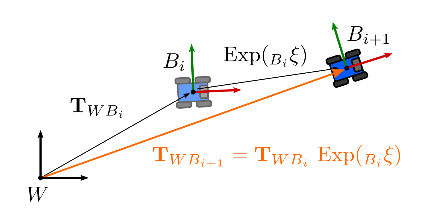
Let us consider a case similar to previous examples in which we were adding a small increment \(_{B_i}\mathbf{\xi}\) to a pose \(\mathbf{T}_{WB_i}\).

\[\begin{equation} \mathbf{T}_{W_i B_{i}} \text{Exp}( _{B_i}\mathbf{\xi}) \end{equation}\]

where we have used the retraction of $\text{SE(3)}$ to add a small increment using the right-hand convention as GTSAM does.

However, for some applications we can be interested in applying a correction from the left:

\[\begin{equation} \mathbf{T}_{W_{i+1} B} = \text{Exp}( _{W_i}\mathbf{\xi}) \mathbf{T}_{W_i B_i} \end{equation}\]

Please note that this case is different to the example in the previous post in which we had the frames inverted. Here we are effectively applying a correction on the world frame.

We are interested in finding out a correction on the body that can lead to the same result that a correction applied on the right. For that specific correction both formulations would be effectively representing the same pose but using different reference frames. This is shown in the next figure:

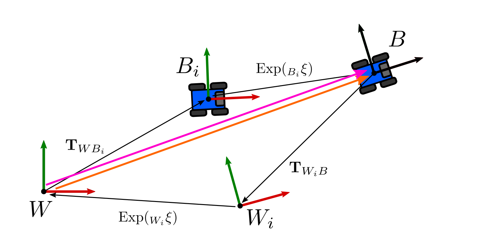
In order to find it, we can write an equivalence between corrections applied on the body frame and the world frame as follows:

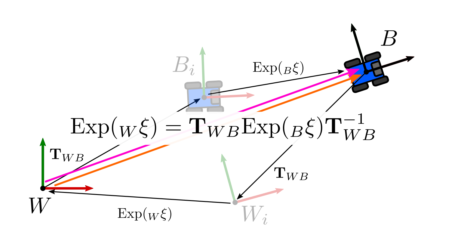
\[\begin{equation} \text{Exp}( _{W}\mathbf{\xi}) \mathbf{T}_{WB} = \mathbf{T}_{WB} \text{Exp}( _{B}\mathbf{\xi}) \end{equation}\]

We dropped the time-related indices for simplicity, since this is a geometric relationship. In order to satisfy this condition, the incremental change we applied on the left-hand side, i.e in the world frame, \(_{W}\mathbf{\xi}\) must be given by:

\[\begin{equation} \text{Exp}( _{W}\mathbf{\xi}) = \mathbf{T}_{WB} \text{Exp}( _{B}\mathbf{\xi}) \mathbf{T}_{WB}^{-1} \end{equation}\]

which we obtained by isolating the term. The expression on the right-hand side is known as the adjoint action of $\text{SE(3)}$. This relates increments applied on the left to ones applied on the right.

For our purposes, it is useful to use an equivalent alternative expression that applies directly to elements from the tangent space (Solà et al. gives a more complete derivation as a result of some properties we omitted here):

\[\begin{equation} \text{Exp}( _{W}\mathbf{\xi}) \mathbf{T}_{WB_i} = \mathbf{T}_{WB_i} \text{Exp}( \text{Ad}_{T_{WB_i}^{-1}} {_{W}}\mathbf{\xi}) \end{equation}\]

where \(\text{Ad}_{T_{WB_i}^{-1}}\) is known as the adjoint matrix or adjoint of \(T_{WB_i}^{-1}\). The adjoint acts over elements of the tangent space directly, changing their reference frame. Please note that the same subindex cancelation applies here, so we can confirm that the transformations are correctly defined.

We can also interpret this as a way to consistently move increments applied on the left-hand side (in world frame) to the right-hand side (body frame), which is particularly useful to keep the right-hand convention for the retractions and probability distributions consistent. This is the main property we will use in the next sections to define some covariance transformations, and it is already implemented in Pose3 as AdjointMap.

Distribution of the inverse

As a first example on how the adjoint helps to manipulate covariances, let us consider the case in which we have the solution of a factor graph, with covariances defined in the body frame as we have discussed previously. We are interested in obtaining an expression to express the covariance in the world frame:

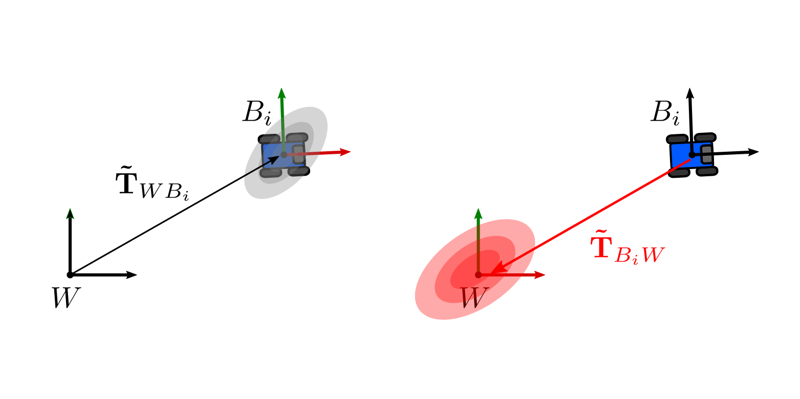
The distribution of the pose assuming Gaussian distribution will be expressed by:

\[\begin{equation} \mathbf{\tilde{T}}_{WB} = \mathbf{T}_{WB} \text{Exp}( _{B}\mathbf{\eta}) \end{equation}\]

with \(_{B}\mathbf{\eta}\) zero-mean Gaussian noise with covariance $\Sigma_{B}$ as before. The distribution of the inverse can be computed by inverting the expression:

\[\begin{align} (\mathbf{\tilde{T}}_{WB})^{-1} & = (\mathbf{T}_{WB} \text{Exp}( _{B}\mathbf{\eta}) )^{-1}\\ & = (\text{Exp}( _{B}\mathbf{\eta}) )^{-1}\ \mathbf{T}_{WB}^{-1}\\ & = \text{Exp}(- _{B}\mathbf{\eta}) \ \mathbf{T}_{WB}^{-1} \end{align}\]

However, the noise is defined on the left, which is inconvenient because is still a covariance in the body frame, but it is also inconsistent with right-hand convention. We can move it to the right using the adjoint:

\[\begin{equation} (\mathbf{\tilde{T}}_{WB})^{-1} = \ \mathbf{T}_{WB}^{-1}\ \text{Exp}(- \text{Ad}_{\mathbf{T}_{WB}} {_{B}}\mathbf{\eta}) \end{equation}\]

This is a proper distribution following the right-hand convention, which defines the covariance in the world frame. The covariance of the inverse is then given by:

\[\begin{equation} \Sigma_{W} = \text{Ad}_{\mathbf{T}_{WB}} \Sigma_B \text{Ad}_{\mathbf{T}_{WB}}^{T} \end{equation}\]

Distribution of the composition

A different case is if we have the distribution of a pose \(\mathbf{\tilde{T}}_{WB_i}\) and we also have an increment given by another distribution \(\mathbf{\tilde{T}}_{B_i B_{i+1}}\). By doing some algebraic manipulation, we can determine the distribution of the composition \(\mathbf{\tilde{T}}_{WB_{i+1}}\). This is useful when doing dead reckoning for instance:

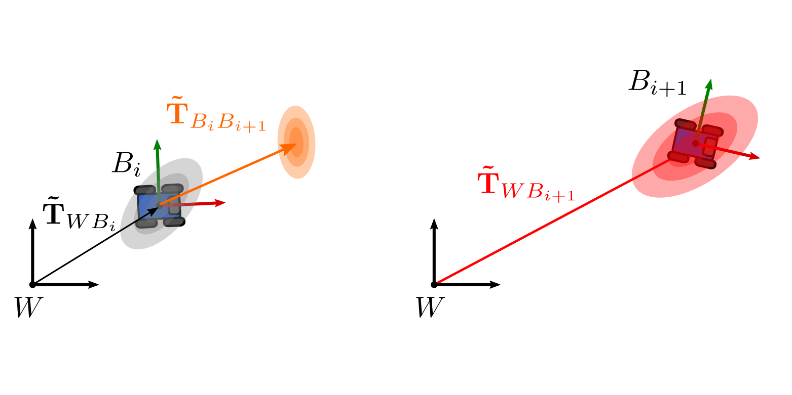
We can determine the distribution of the composition (and its covariance) if we follow a similar formulation as before:

\[\begin{align} \mathbf{\tilde{T}}_{WB_{i+1}} &= \mathbf{\tilde{T}}_{WB_i} \mathbf{\tilde{T}}_{B_i B_{i+1}}\\ &= \mathbf{T}_{WB_i} \text{Exp}( _{B_i}\mathbf{\eta})\ \mathbf{T}_{B_i B_{i+1}} \text{Exp}( _{B_{i+1}}\mathbf{\eta}) \end{align}\]

Analogously, we need to move the noise \(_{B_i}\mathbf{\eta}\) to the right, so as to have the transformations to the left (which represent the mean of the distribution), and the noises to the right (that encode the covariance). We can use the adjoint again:

\[\begin{equation} \mathbf{\tilde{T}}_{WB_i} = \mathbf{T}_{WB_i} \ \mathbf{T}_{B_i B_{i+1}} \text{Exp}(\text{Ad}_{\mathbf{T}_{B_i B_{i+1}}^{-1}} {_{B_i}}\mathbf{\eta})\ \text{Exp}( _{B_{i+1}}\mathbf{\eta}) \end{equation}\]

However, we cannot combine the exponentials because that would assume commutativity in the group that does not hold for $\text{SE(3)}$ as we discussed previously. Still, it is possible to use some approximations (also discussed in Mangelson’s) to end up with the following expressions for the covariance of the composition:

\[\begin{equation} \Sigma_{B_{i+1}} = \text{Ad}_{\mathbf{T}_{B_i B_{i+1}}^{-1}} \Sigma_{B_{i}} \text{Ad}_{\mathbf{T}_{B_i B_{i+1}}^{-1}}^{T} + \Sigma_{B_{i+1}} \end{equation}\]

Additionally, if we consider that the poses are correlated and then the covariance of the joint distribution is given by:

\[\begin{equation} \begin{bmatrix} \Sigma_{B_{i}} & \Sigma_{B_{i}, B_{i+1}} \\ \Sigma_{B_{i}, B_{i+1}}^{T} & \Sigma_{B_{i+1}} \end{bmatrix} \end{equation}\]

We have that the covariance of the composition is:

\[\begin{equation} \begin{split} \Sigma_{B_{i+1}} &= \text{Ad}_{\mathbf{T}_{B_i B_{i+1}}^{-1}} \Sigma_{B_{i}} \text{Ad}_{\mathbf{T}_{B_i B_{i+1}}^{-1}}^{T} + \Sigma_{B_{i+1}} \\ &\qquad + \text{Ad}_{\mathbf{T}_{B_i B_{i+1}}^{-1}} \Sigma_{B_{i}, B_{i+1}} + \Sigma_{B_{i}, B_{i+1}}^{T} \text{Ad}_{\mathbf{T}_{B_i B_{i+1}}^{-1}}^{T} \end{split} \end{equation}\]

Distribution of the relative transformation

Lastly, it may be the case that we have the distributions of two poses expressed in the same reference frame, and we want to compute the distribution of the relative transformation between them. For example, if we have an odometry system that provides estimates with covariance and we want to use relative measurements as factors for a pose graph SLAM system, we will need the mean and covariance of the relative transformation.

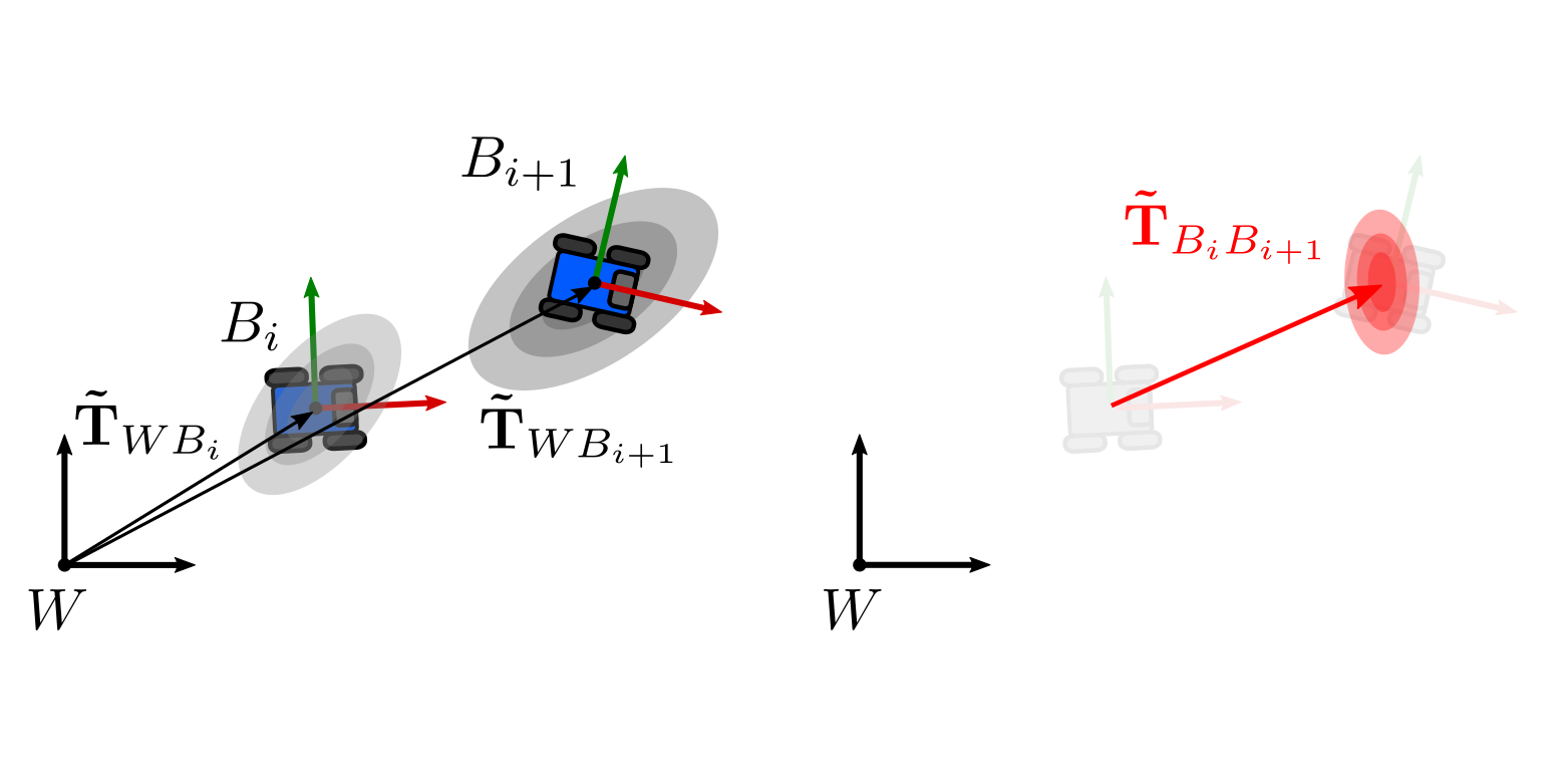
To determine it we follow the same algebraic procedure:

\[\begin{align} \mathbf{\tilde{T}}_{B_i B_{i+1}} &= \mathbf{\tilde{T}}_{W B_{i}}^{-1} \mathbf{\tilde{T}}_{WB_{i+1}}\\ &= \left( \mathbf{T}_{WB_i} \text{Exp}( _{B_i}\mathbf{\eta}) \right)^{-1} \ \mathbf{T}_{WB_{i+1}} \text{Exp}( _{B_{i+1}}\mathbf{\eta})\\ &= \text{Exp}(- _{B_i}\mathbf{\eta}) \ \mathbf{T}_{WB_i}^{-1} \ \mathbf{T}_{WB_{i+1}} \text{Exp}( _{B_{i+1}}\mathbf{\eta}) \end{align}\]

Similarly, we use the adjoint to move the exponential twice:

\[\begin{align} \mathbf{\tilde{T}}_{B_i B_{i+1}} &= \mathbf{T}_{WB_i}^{-1} \text{Exp}(- \text{Ad}_{\mathbf{T}_{WB_i}} \ {_{B_i}}\mathbf{\eta}) \ \mathbf{T}_{WB_{i+1}} \text{Exp}( _{B_{i+1}}\mathbf{\eta})\\ &= \mathbf{T}_{WB_i}^{-1} \ \mathbf{T}_{WB_{i+1}} \ \text{Exp}(- \text{Ad}_{\mathbf{T}_{WB_{i+1}}^{-1}} \ \text{Ad}_{\mathbf{T}_{WB_i}}\ {_{B_i}}\mathbf{\eta}) \ \text{Exp}( _{B_{i+1}}\mathbf{\eta}) \end{align}\]

Hence, the following covariance holds for the relative pose assuming independent poses:

\[\begin{equation} \Sigma_{B_{i+1}} = \left(\text{Ad}_{\mathbf{T}_{WB_{i+1}}^{-1}} \text{Ad}_{\mathbf{T}_{WB_i}} \right) \Sigma_{B_{i}} \left(\text{Ad}_{\mathbf{T}_{WB_{i+1}}^{-1}} \text{Ad}_{\mathbf{T}_{WB_i}}\right)^{T} + \Sigma_{B_{i+1}} \end{equation}\]

A problem that exist with this expression, however, is that by assuming independence the covariance of the relative poses will be larger than the covariance of each pose separately. This is consistent with the 1-dimensional case in which we compute the distribution of the difference of independent Gaussians, in which the mean is the difference while the covariance gets increased. However, this is not the result that we would want, since our odometry factors will degrade over time.

Mangelson et al. showed that if some correlations exists (as we showed for the composition example) and it is explicitly considered in the computation, the estimates get more accurate and the covariance is not over or underestimated. The corresponding expression that complies with GTSAM is then:

\[\begin{equation} \begin{split} \Sigma_{B_{i+1}} & = \left(\text{Ad}_{\mathbf{T}_{WB_{i+1}}^{-1}} \text{Ad}_{\mathbf{T}_{WB_i}} \right) \Sigma_{B_{i}} \left(\text{Ad}_{\mathbf{T}_{WB_{i+1}}^{-1}} \text{Ad}_{\mathbf{T}_{WB_i}}\right)^{T} + \Sigma_{B_{i+1}} \\ &\qquad - \left(\text{Ad}_{\mathbf{T}_{WB_{i+1}}^{-1}} \text{Ad}_{\mathbf{T}_{WB_i}} \right) \Sigma_{B_{i} B_{i+1}} - \Sigma_{B_{i} B_{i+1}}^{T} \left(\text{Ad}_{\mathbf{T}_{WB_{i+1}}^{-1}} \text{Ad}_{\mathbf{T}_{WB_i}} \right)^{T} \end{split} \end{equation}\]

Conclusions

In this final post we reviewed the concept of the adjoint of a Lie group to explain the relationship between increments applied on the left with increments applied on the right. This was the final piece we needed to ensure that our estimates are consistent with the conventions used in GTSAM.

We also presented a few expressions to operate distributions of poses. While they were presented previously in the literature, we showed general guidelines on how to manipulate the uncertainties to be consistent with the frames and convention we use.

Acknowledgments

I would like to thank again the interesting discussions originated in the gtsam-users group. Stefan Gächter guided a rich conversation doing some important questions that motivated the idea of writing this post.

Coincidently, similar discussions we had at the Dynamic Robot Systems group at the University of Oxford were aligned with the topics discussed here and facilitated the writing process. Special thanks to Yiduo Wang and Milad Ramezani for our conversations, derivation and testing of the formulas for the covariance of relative poses presented here, Marco Camurri for feedback on the notation and proofreading, and Maurice Fallon for encouraging to write this post.

Finally, thanks to Frank Dellaert, José Luis Blanco-Claraco, and John Lambert for proofreading the posts and their feedback, as well as Michael Bosse for providing insightful comments to ensure the consistency of the topics presented here.