Author: Matias Mattamala

Introduction

In these posts I will review some general aspects of optimization-based state estimation methods, and how to input and output consistent quantities and uncertainties, i.e, covariance matrices, from them. We will take a (hopefully) comprehensive tour that will cover why we do the things the way we do, aiming to clarify some uncertain things about working with covariances. We will see how most of the explanations naturally arise by making explicit the definitions and conventions that sometimes we implicitly assume when using these tools.

They summarize and extend some of the interesting discussions we had in the gtsam-users group. We hope that such space will continue to bring to the table relevant questions shared by all of us.

A simple example: a pose graph

As a motivation, we will use a similar pose graph to those used in other GTSAM examples:

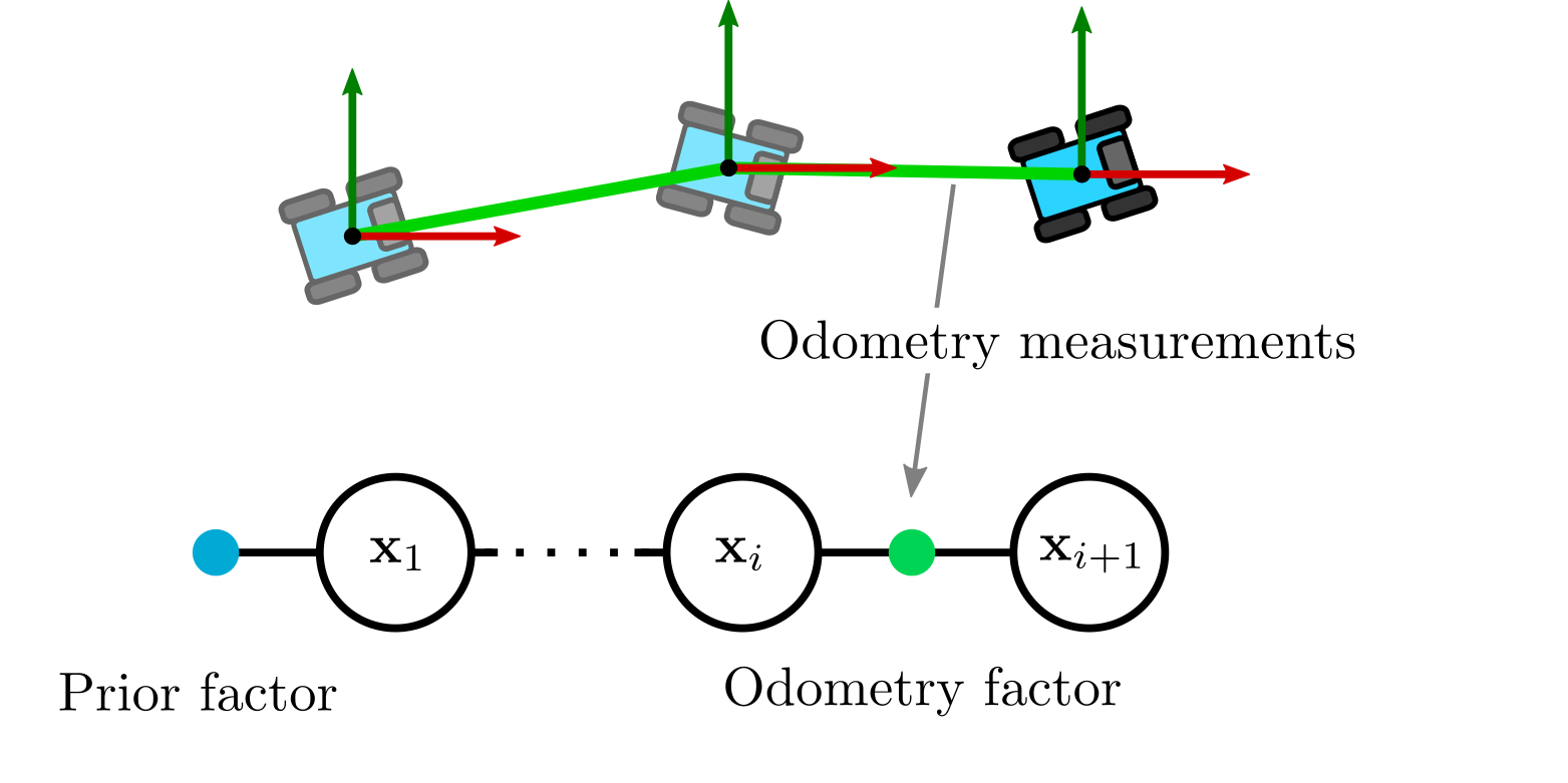
To start, we will consider that the variables in the graph \(\mathbf{x}_i\) correspond to positions \({\mathbf{x}_{i}} = (x,y) \in \mathbb{R}^2\). The variables are related by a linear model given by a transition matrix \(\mathbf{A}_{i}\) and a constant term \(\mathbf{b}_{i} = (b_x, b_y)\), which can be obtained from some sensor such as a wheel odometer. We can then establish the following relationship between variables \(i\) and \(i+1\):

\[\begin{equation} \mathbf{x}_{i+1} = \mathbf{A}_{i} \mathbf{x}_i + \mathbf{b}_i \end{equation}\]

However, we know that in reality things do not work that way, and we will usually have errors produced by noise in our sensors or actuators. The most common way to address this problem is adding some zero-mean Gaussian noise \(\eta_i\sim Gaussian(\mathbf{0}_{2\times1}, \Sigma_i)\) to our model to represent this uncertainty:

\[\begin{equation} \mathbf{x}_{i+1} = \mathbf{A}_{i}\mathbf{x}_i + \mathbf{b}_i + \eta_i \end{equation}\]

We can recognize here the typical motion or process model we use in Kalman filter for instance, that describes how our state evolves. We say that the noise we introduced on the right side states that our next state \(\mathbf{x}_{i+1}\) will be around \(\mathbf{A}_{i}\mathbf{x}_i + \mathbf{b}_i\), and the covariance matrix \(\Sigma_i\) describes the region where we expect \(\mathbf{x}_{i+1}\) to lie.

We can also notice that with a bit of manipulation, it is possible to establish the following relationship:

\[\begin{equation} \eta_i = \mathbf{x}_{i+1} - \mathbf{A}_{i}\mathbf{x}_i - \mathbf{b}_i \end{equation}\]

This is an important expression because we know that the left-hand expression follows a Gaussian distribution. But since we have an equivalence, the right-hand term must do as well. We must note here that what distributes as a Gaussian is neither \(\mathbf{x}_{i}\) nor \(\mathbf{x}_{i+1}\), but the difference \((\mathbf{x}_{i+1} - \mathbf{A}_{i}\mathbf{x}_i - \mathbf{b}_i)\). This allows us to use the difference as an odometry factor that relates \(\mathbf{x}_i\) and \(\mathbf{x}_{i+1}\) probabillistically in our factor graph:

\[\begin{equation} (\mathbf{x}_{i+1} - \mathbf{A}_{i}\mathbf{x}_i - \mathbf{b}_i) \sim Gaussian(\mathbf{0}_{2\times1}, \Sigma_i) \end{equation}\]

Analyzing the solution

Solving the factor graph using the previous expression for the odometry factors is equivalent to solve the following least squares problem under the assumption that all our factors are Gaussian and we use maximum-a-posteriori (MAP) estimation, which is fortunately our case:

\[\begin{equation} \mathcal{X}^{*} = \argmin\displaystyle\sum_{i} || \mathbf{A}_i \mathbf{x}_{i} + \mathbf{b}_{i} - {\mathbf{x}_{i+1}} ||^{2}_{\Sigma_i} \end{equation}\]

Please note here that while we swapped the terms in the factor to be consistent with GTSAM’s documentation, it does not affect the formulation since the term is squared.

The previous optimization problem is linear with respect to the variables, hence solvable in closed form. By differentiating the squared cost, setting it to zero and doing some manipulation, we end up with the so-called normal equations, which are particularly relevant for our posterior analysis:

\[\begin{equation} \mathbf{A}^{T} \Sigma^{-1} \mathbf{A}\ \mathcal{X}^{*} = \mathbf{A}^{T} \Sigma^{-1} \mathbf{b} \end{equation}\]

where the vector $\mathcal{X}^{*}$ stacks all the variables in the problem, $\mathbf{A}$ is a matrix that stacks the linear terms in the factors, and $\mathbf{b}$ does the same for the constant vector terms.

First point to note here is that finding the solution $\mathcal{X}^{*}$ requires to invert the matrix $\mathbf{A}^{T} \Sigma^{-1} \mathbf{A}$, which in general is hard since it can be huge and dense in some parts. However we know that there are clever ways to solve it, such as iSAM and iSAM2 that GTSAM already implements, which are covered in this comprehensive article by Frank Dellaert and Michael Kaess.

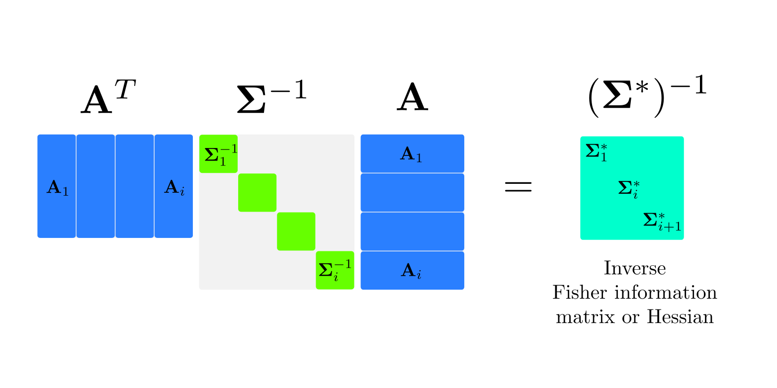
Our interest in this matrix, though, known as Fisher information matrix or Hessian (since it approximates the Hessian of the original quadratic cost), is that its inverse \(\Sigma^{*} = (\mathbf{A}^{T} \Sigma^{-1} \mathbf{A})^{-1}\) also approximates the covariance of our solution - known as Laplace approximation in machine learning (Bishop (2006), Chap. 4.4). This is a quite important result because by solving the factor graph we are not only recovering an estimate of the mean of the solution but also a measure of its uncertainty. In GTSAM, the Marginals class implements this procedure and a example can be further explored in the tutorial.

As a result, we can say that after solving the factor graph the probability distribution of the solution is given by \(Gaussian(\mathcal{X}^{*}, \Sigma^{*})\).

Getting nonlinear

The previous pose graph was quite simple and probably not applicable for most of our problems. Having linear factors as the previous one is an impossible dream for most of the applications. It is more realistic to think that our state \(i+1\) will evolve as a nonlinear function of the state $i$ and the measurements, which is more general than the formerly assummed linear model \(\mathbf{A}_{i} \mathbf{x}_i + \mathbf{b}_i\):

\[\begin{equation} \mathbf{x}_{i+1} = f(\mathbf{x}_i) \end{equation}\]

Despite nonlinear, we can still say that our mapping has some errors involved, which are embeded into a zero-mean Gaussian noise that we can simply add as before:

\[\begin{equation} \mathbf{x}_{i+1} = f(\mathbf{x}_i) + \eta_i \end{equation}\]

Following a similar procedure as before isolating the noise, we can reformulate the problem as the following nonlinear least squares (NLS) problem:

\[\begin{equation} \mathcal{X} = \argmin \displaystyle\sum_i || f(\mathbf{x}_i) - \mathbf{x}_{i+1} ||^2_{\Sigma_i} \end{equation}\]

Since the system is not linear with respect to the variables anymore we cannot solve it in close form. We need to use nonlinear optimization algorithms such as Gauss-Newton, Levenberg-Marquardt or Dogleg. They will try to approximate our linear dream by linearizing the residual with respect to some linearization or operation point given by a guess \(\mathcal{\bar{X}}^{k}\) valid at iteration $k$:

\[\begin{equation} f(\mathbf{x}_i) \approx f(\mathbf{\bar{x}}^{k}) + \mathbf{H}(\mathbf{\bar{x}}^{k})\mathbf{x}_i = \mathbf{b}_k + \mathbf{H}^k \mathbf{x}_i \end{equation}\]

where \(\mathbf{H}(\mathbf{\bar{x}}^{k})\) denotes the Jacobian of \(f(\cdot)\) evaluated at the linearization point \(\mathbf{\bar{x}}^{k}\). Hence the problem becomes:

\[\begin{equation} \delta\mathcal{X}^{k}= \argmin \displaystyle\sum_i || \mathbf{H}^k\mathbf{x}_i + \mathbf{b}_i - \mathbf{x}_{i+1} ||^2_{\Sigma_i^k} \end{equation}\]

It is important to observe here that we are not obtaining the global solution $\mathcal{X}$, but just a small increment $\delta\mathcal{X}^{k}$ that will allow us to move closer to some minima that depends on the initial values. This linear problem can be solved in closed form as we did before. In fact, the normal equations now become something similar to the linear case:

\[\begin{equation} \label{nonlinear-normal-equations} (\mathbf{H}^k)^{T} (\Sigma^{k})^{-1}\ \mathbf{H}^k\ \delta\mathcal{X} = (\mathbf{H}^k)^{T} (\Sigma^{k})^{-1} \mathbf{b} \end{equation}\]

where \(\mathbf{H}^k\) is built by stacking the Jacobians at iteration $k$. The solution $\delta\mathcal{X}^{k}$ will be used to update our current solution at iteration $k$ using the update rule:

\[\begin{equation} \mathcal{X}^{k+1} = \mathcal{X}^k + \delta\mathcal{X}^{k} \end{equation}\]

where \(\mathcal{X}^{k+1}\) corresponds to the best estimate so far, and can be used as a new linearization point for a next iteration.

Similarly, the expression on the left-hand side \(\Sigma^{k+1} = ((\mathbf{H}^k)^{T} (\Sigma^{k})^{-1} \mathbf{H}^k)^{-1}\) also corresponds to the Fisher information or Hessian as before, but with respect to the linearization point. This is quite important because both the best solution so far $\mathcal{X}^{k+1}$ and its associated covariance $\Sigma^{k+1}$ will be valid only at this linearization point and will change with every iteration of the nonlinear optimization. But understanding this, we still can say that at iteration $k+1$ our best solution will follow a distribution $Gaussian(\mathcal{X}^{k+1}, \Sigma^{k+1})$.

Conclusions

In this first post we reviewed the basics ideas to solve factor graphs and extract estimates from them. We showed how the linear problem described by the normal equations not only allows us to find the solution, but also encodes information about its covariance - given by the inverse of the Fisher information matrix. Additionally, in the context of nonlinear problems, we showed how such covariance is only valid around the linearization point.

In our next post we will review how these ideas generalize when we are not estimating vector variables anymore but other objects such as rotation matrices and rigid-body transformations - generally known as manifolds. While this will introduce a bit of complexity not only in the maths but also the notation, by being explicit about our conventions we will be able to consistently solve a wider set of problems usually found in robotics and computer vision.