Authors: Connor Holmes, Sven Lilge, Zi Cong Guo, Frank Dellaert, and Timothy D. Barfoot

In modern robotics, we often represent trajectories using discrete-time elements, but many real-world scenarios benefit from a continuous representation. Whether you are dealing with high-rate asynchronous sensors, rolling-shutter cameras, or the need to sample a trajectory at arbitrary times for control and planning, continuous-time (CT) estimation provides a principled solution.

The two main approaches for CT estimation to date involve either parametric approaches, such as splines, or non-parametric ones, such as Gaussian processes (GPs). While GTSAM is traditionally used for discrete-time factor graph problems, it now features powerful capabilities for GP-based continuous-time estimation, accompanying our recent paper.

An example of GP-based CT trajectory is shown below. The trajectory specifically includes states $\mathbf{x}$ (e.g., position or pose of a robot over time) at discrete times $t_k$ (typically when measurements occur), but retains the ability to query the mean and covariance of the state at any arbitrary time $\tau$ through the interpolation capabilities of the underlying Gaussian process.

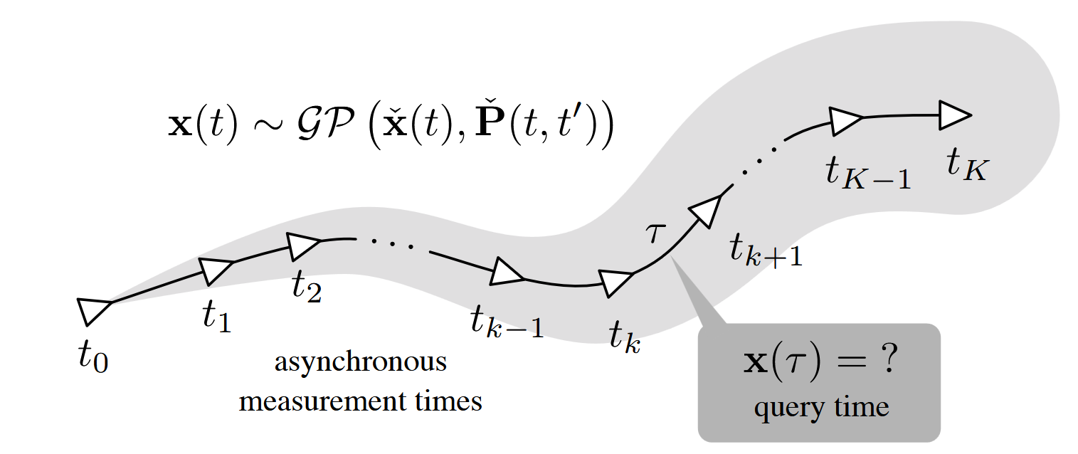
A core insight that we share in our recent paper is that querying such a trajectory at any time is mathematically equivalent to an application of the standard factor-graph elimination algorithm. This perspective not only makes the math more intuitive but also reveals how to perform efficient $O(1)$ interpolation for both the state’s mean and covariance.

GTSAM now features built-in capabilities to carry out GP-based continuous-time estimation within the existing factor graph framework.

New GTSAM Features

We introduce several key components to GTSAM for performing CT estimation on vector spaces (Point1, Point2, Point3) and Lie groups (Pose2, Pose3):

• StateData: A custom struct that links poses, velocities, and timestamps for a given state.
• WnoaMotionFactor: A binary motion prior factor that connects neighboring pose and velocity pairs based on a White-Noise-on-Acceleration (WNOA) model. This prior smooths the trajectory by assuming constant velocities and endows the estimation with a continuous-time GP interpretation.
• WnoaInterpFactor: A powerful wrapper factor that allows you to add measurements to your graph at arbitrary timestamps, even those not included in the main graph. It internally handles the GP-interpolation, linking asynchronous data to the discrete states you are optimizing.
• interpolateFactorGraph: A convenience function that can automatically convert a standard factor graph into a reduced, equivalent graph where selected states are interpolated, significantly reducing the size of the optimization problem.
• Post-Solve Querying: Functions like updateInterpValues and updateInterpValuesWithCovariance allow you to query the full, smooth trajectory and its uncertainty after the main optimization is complete.

An Example on $SE(3)$

To see these tools in action, let’s consider a simple $SE(3)$ trajectory example.

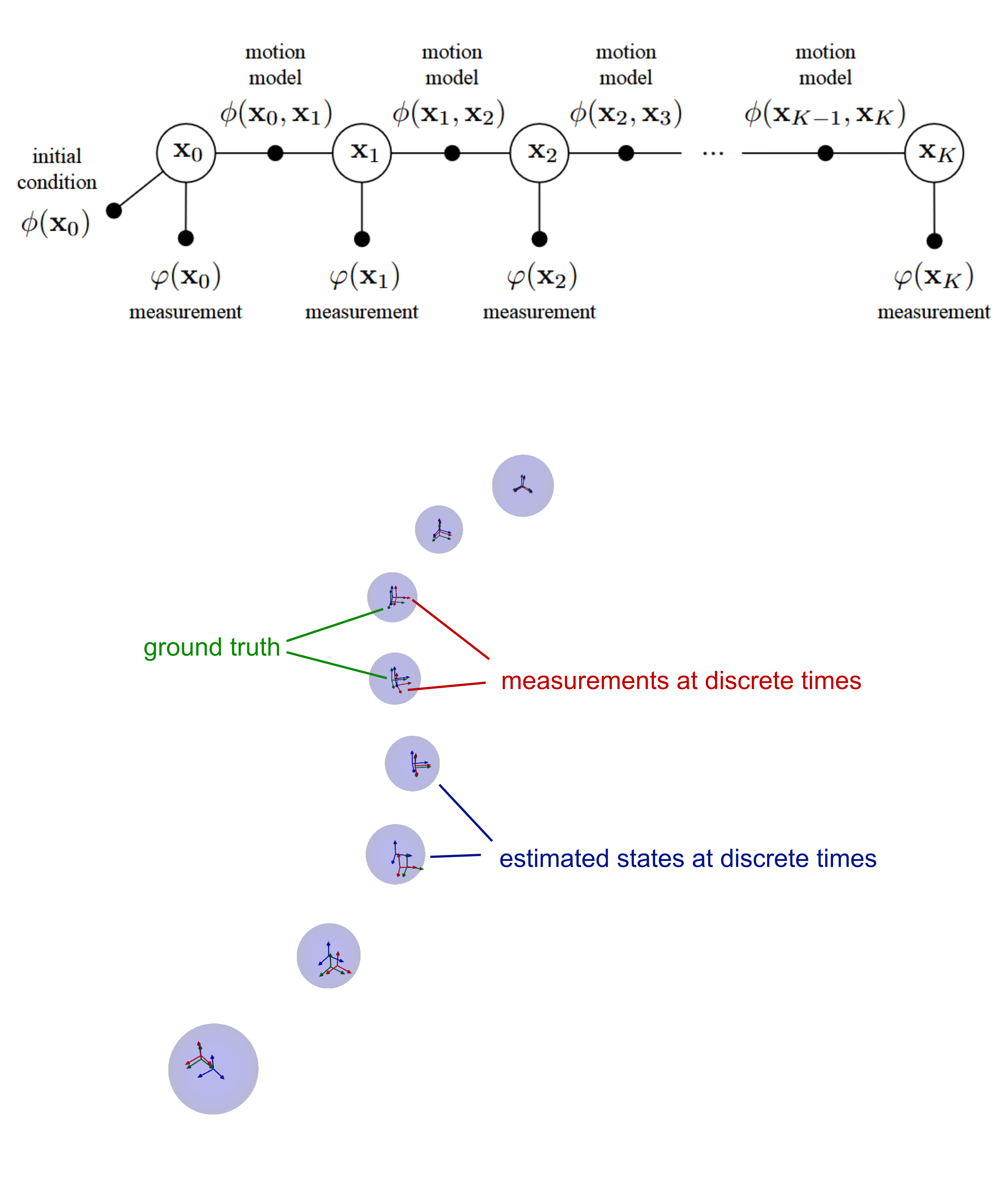
The most straightforward workflow is to define a trajectory by creating StateData entries for the states at discrete times and linking them with the binary WnoaMotionFactor. We can then add measurements to any of those states at discrete times, such as pose or velocity observations. In this example, we use pose measurements. The resulting graph contains both binary and unary factors, and solving it with standard GTSAM solvers gives us the mean and covariance of each state, as shown in the figure below.

We can now use the new GTSAM functionalities to additionally query the mean and covariance of the trajectory at any arbitrary time. The figure below shows a much denser trajectory with a smooth state. States at queried times can be recovered by drawing an analogy to factor-graph elimination, as illustrated in the figure. This lets us query the trajectory after solving the discrete problem at any time, which is useful for downstream tasks such as planning and control.

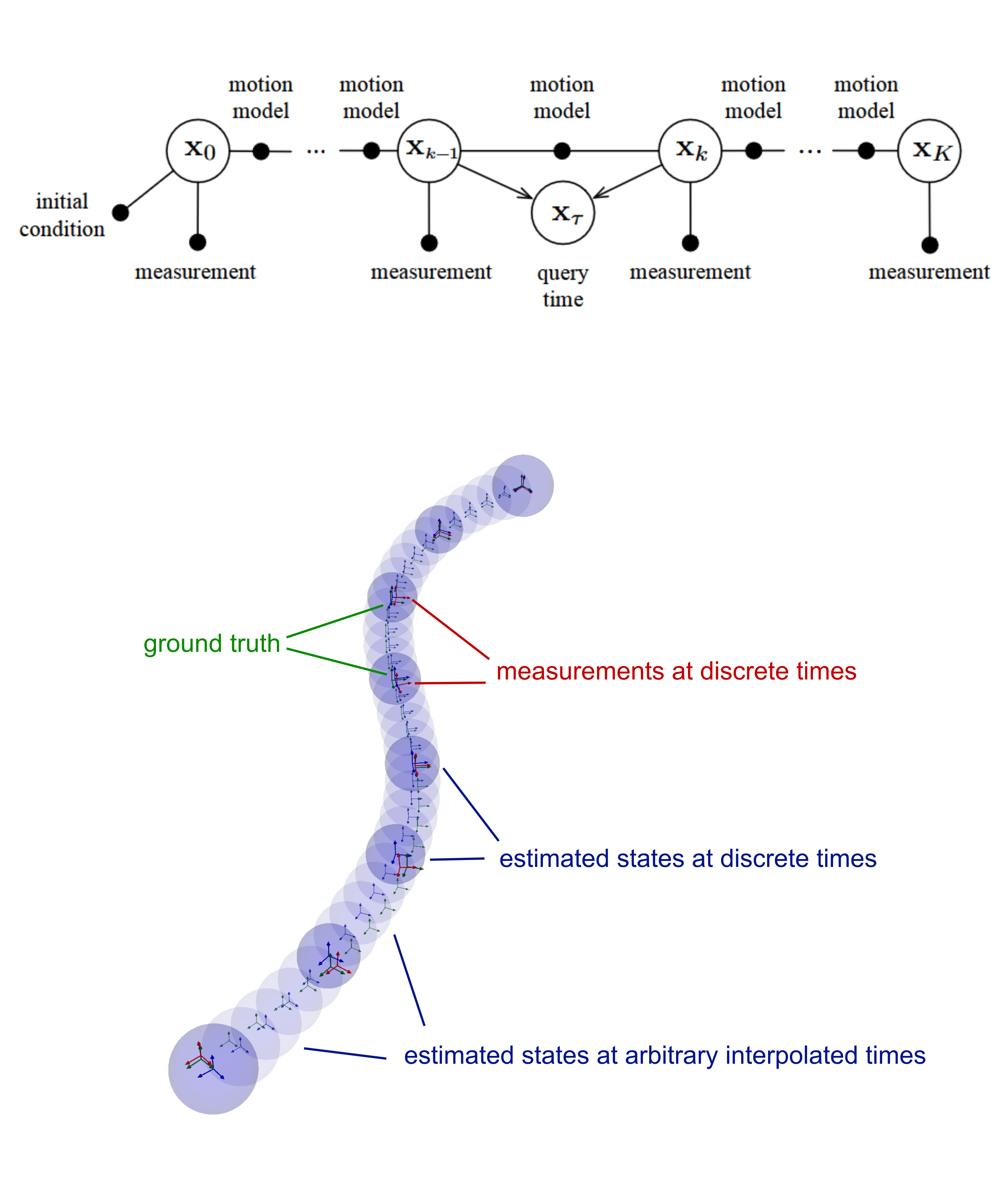
Finally, we are not restricted to measurements, or any other factors, that align exactly with the optimization states at discrete times.

As illustrated in the figure below, suppose we receive a measurement at an arbitrary time $\tau$. In a traditional setup (left), we would need to insert a new state $\mathbf{x}_\tau$ into the optimization graph. Instead, we can conceptually eliminate $\mathbf{x}_\tau$ using the GP motion model. This elimination produces two distinct components (right):

1. A conditional density $p(\mathbf{x}_\tau \mid \mathbf{x}_k, \mathbf{x}_{k-1})$ representing the eliminated state $\mathbf{x}_\tau$ (shown in gray).
2. A new measurement factor $\phi_y(\mathbf{x}_{k-1}, \mathbf{x}_k)$ that depends solely on the two neighboring bounding states, $\mathbf{x}_{k-1}$ and $\mathbf{x}_k$.

In GTSAM, we implement this mechanism using the wrapper factor WnoaInterpFactor. It converts a factor at an arbitrary time into this neighboring-state factor, allowing GTSAM to optimize the trajectory while correctly accounting for exact time associations via GP interpolation.

The bottom of the figure demonstrates this in practice. This formulation is especially useful when measurements are asynchronous or arrive at high rates (shown in red). Rather than including states in the graph for every single measurement, we only need to optimize a subset of discrete states (dark blue) at a lower rate, such as 10 Hz. The wrapper factor relies on GP interpolation to correctly relate the asynchronous measurements to the discrete states, effectively enabling exact continuous-time interpolation during the solve rather than only post-solve.

Takeaway

The integration of GP-based continuous-time estimation into GTSAM provides a flexible, modular framework that maintains the library’s standard workflow. It allows practitioners to handle asynchronous sensor data in a principled way and reduce problem sizes without sacrificing the fidelity of the continuous trajectory.

Additional Reading

For a deeper dive into the theory and broader context of these methods, we recommend reading our recent paper, “Smoothing Out the Edges: Continuous-Time Estimation with Gaussian Process Motion Priors on Factor Graphs”.

You can find more details on the example used in this blogpost in our GTSAM Example Notebook and interactive Google Colab Notebook. Please also visit our GitHub Repository for further real-world robotics examples. These specifically include:

1. 1D (Giant Glass of Milk): A mobile robot driving back and forth in a straight line, demonstrating basic smoothing.
2. 2D (Lost in the Woods): SLAM and localization for a wheeled robot using asynchronous landmark observations, showing problem-size reduction via aggressive interpolation.
3. 3D (Starry Night): $SE(3)$ localization using a stereo camera and IMU, illustrating high-fidelity trajectory recovery with 80% fewer states in the main solve by relying on GP interpolation.

Disclosure: AI was used to help draft this post.