The Manifold Kalman Filter Hierarchy, Part 1
GTSAM Posts
Authors: Frank Dellaert, Scott Baker
GTSAM now has a small but useful hierarchy of Kalman filters for states that do not live in a plain vector space. This post is the first in a short series on that hierarchy. Here I will start with the classes that are already useful today for manifold and Lie-group filtering:
ManifoldEKFLieGroupEKFInvariantEKFLeftLinearEKF
Part 2 will cover the newer equivariant filters.
Why a hierarchy?
The classical EKF assumes the state is a vector in $R^n$. That is fine for many systems, but it is a bad fit for rotations, poses, and navigation states. In those cases the state lives on a manifold, and often on a Lie group, so the filter needs to respect that geometry.
GTSAM’s new hierarchy separates the common update logic from increasingly structured prediction models:
ManifoldEKFhandles the generic case: state on a manifold, covariance in the tangent space.LieGroupEKFspecializes prediction to Lie groups with state-dependent dynamics.InvariantEKFis a particularly important case where the prediction is pure group composition and the linearized error dynamics become state independent.LeftLinearEKFgeneralizes that with a left-linear prediction model $X_{k+1} = W \phi(X_k) U$.
The best single starting point in the tree today is the navigation note EKF-variants.md, and in the GTSAM context the main motivation is really NavState: once you want filtering on rotation, position, and velocity together, the plain vector-space EKF viewpoint starts to become awkward.
1. ManifoldEKF
ManifoldEKF is the base class. It does not assume a vector-space state. Instead, it stores:
- a state $X$ on a manifold $M$
- a covariance $P$ in the tangent space at $X$
That is the right abstraction for objects like Unit3, Pose2, Pose3, Rot3, and NavState. It also works perfectly well for ordinary vector states such as gtsam::Vector, so this is not only about fancy geometry.
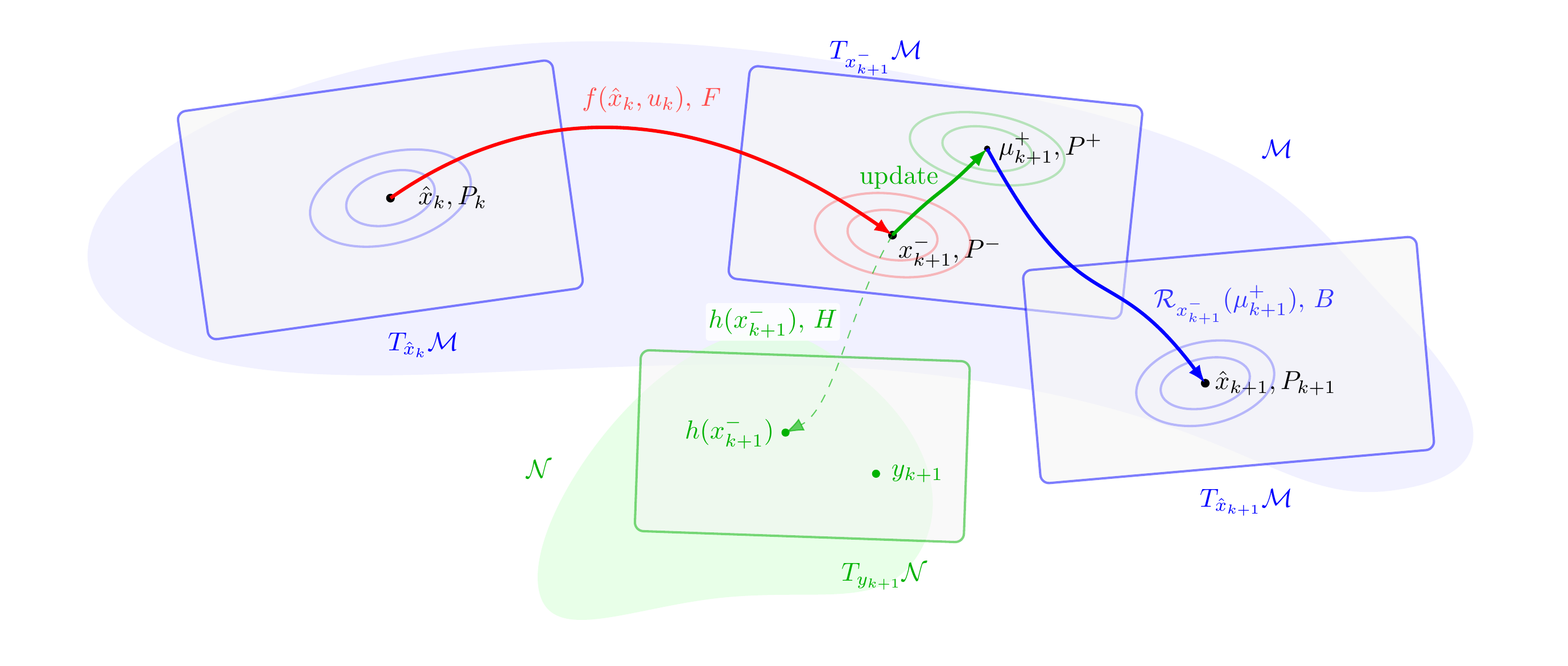
The predict step is intentionally minimal: you supply the next state and the transition Jacobian in local coordinates,
\[X_{k+1} = X_{\text{next}}, \qquad P_{k+1} = F_k P_k F_k^T + Q_k.\]The figure above is a good way to read the algorithm. The red arrow is the predict step on the state manifold, the green arrow is the measurement update in the tangent space, and the blue arrow is the reset step that moves the corrected tangent-space estimate back to the manifold.
The tangent spaces are the key point. In the figure, the red prediction moves from $T_{\mu_k}\mathcal{M}$ to the predicted state on the manifold, after which the filter works in the tangent space at that predicted state. The green measurement update uses the measurement tangent space $T_y\mathcal{N}$ together with the predicted state tangent space to compute a correction, producing a corrected estimate in the tangent space at the predicted state. The actual retract happens only in the blue reset step, where that corrected tangent-space estimate is pushed back onto the manifold and the covariance is transported to the new tangent space at the updated state.
This is the core idea behind the whole hierarchy: keep the estimate on the manifold, do uncertainty calculations in the tangent space, and transport covariance correctly when the base point changes.
Useful places to look:
- Header: ManifoldEKF.h
- Tests: testManifoldEKF.cpp
The tests are worth a look because they show the class on both Unit3 and Pose2, which makes the base abstraction very concrete.
2. LieGroupEKF
LieGroupEKF is the next step up. It covers the important middle case: Lie-group states with state-dependent dynamics.
This is the right abstraction when the state lives on a Lie group, but the prediction model still depends on the current state estimate. In other words, it keeps the geometry of the state space, but does not yet assume the extra symmetry structure that makes invariant filtering possible.
Useful sources here are:
- Header: LieGroupEKF.h
- Tests: testLieGroupEKF.cpp
- Example: GEKF_Rot3Example.cpp
That example uses a Rot3 state with state-dependent dynamics and a magnetometer update. It shows that not every useful Lie-group filter needs to be invariant.
3. InvariantEKF
InvariantEKF is the most immediately useful class in the current set. It uses the left-invariant prediction structure emphasized by Barrau and Bonnabel; a good entry point is the survey-style tutorial “The Invariant Extended Kalman Filter as a Stable Observer” and the related IEKF papers by Barrau and Bonnabel.
In the simplest view,
\[X_{k+1} = X_k U_k,\]or more generally
\[X_{k+1} = W_k X_k U_k.\]The key payoff is that the error dynamics are state independent. In the basic case implemented here, the linearized propagation Jacobian is
\[F_k = \operatorname{Ad}_{U_k^{-1}},\]so it depends only on the increment $U_k$, not on the current state estimate $X_k$.
This is why invariant filtering tends to be more robust on Lie groups: the error propagation is correct even if the filter state is wrong, which is especially important in transients and at startup.
Our current InvariantEKF is deliberately more restricted than the full theory. For now it focuses on the clean left-invariant prediction cases that fit naturally in the current GTSAM API. That is a narrower target than the IEKF paper treatment, which uses the concept of group-affine dynamics, but it is probably the most useful case to have available first.
For hands-on exploration, start with the notebooks:
- Notebook: InvariantEKF.ipynb
- Notebook: Gal3ImuEKF.ipynb
- Notebook: Gal3ImuExample.ipynb
- Notebook: Gal3ImuASVExample.ipynb
Then look at the concrete repository examples:
- IEKF_SE2Example.cpp: left-invariant filtering on
Pose2with odometry prediction and GPS-like updates - IEKF_NavstateExample.cpp: invariant filtering on
NavStatewith IMU prediction and GPS update
4. LeftLinearEKF
LeftLinearEKF is a later and more general extension of the same line of thinking. In the GTSAM context, the motivation for this extra concept is NavState: it is exactly what lets us model the autonomous part of navigation dynamics cleanly, with velocity driving position through an automorphism before the left and right group increments are applied.
It is for Lie-group systems whose discrete dynamics can be written as
\[X_{k+1} = W_k \, \phi(X_k) \, U_k,\]where $\phi$ is an automorphism of the group.
That is a big word, but for NavState the key idea is simple: position advances by velocity in the autonomous part of the dynamics,
This is directly inspired by the Barrau-Bonnabel paper “Linear Observed Systems on Groups”.
Viewed this way, InvariantEKF is really a special case of LeftLinearEKF: the case where the automorphism part is trivial, so the prediction collapses to group composition. I wanted to introduce InvariantEKF first because it is likely to be the more useful entry point for most users, but mathematically LeftLinearEKF is the more general object.
For hands-on exploration, start with the notebooks:
- Notebook: NavStateImuEKF.ipynb
- Notebook: NavStateImuExample.ipynb
- Notebook: NavStateImuASVExample.ipynb
Then look at the class and tests:
- Class: NavStateImuEKF.h
- Test: testLeftLinearEKF.cpp
So even if you never instantiate LeftLinearEKF directly, it is already paying for itself as the mathematical backbone for more specialized filters.
Part 2
This hierarchy does not stop at invariant filtering. The next step is equivariant filtering, where symmetry is used even more explicitly. GTSAM already has the machinery for that as well, including:
We will cover that in detail in part two.
Disclosure: AI was used to help draft this post.