LOST in Triangulation
GTSAM Posts
Authors: Akshay Krishnan, Sebastien Henry, Frank Dellaert, John Christian
This post introduces the triangulation problem and some commonly used solutions (both optimal and sub-optimal), along with GTSAM code examples. We also discuss a recently proposed linear optimal triangulation method (LOST) and compare its performance to other methods.
TL;DR: LOST can be easily enabled in GTSAM by setting useLOST=True in triangulatePoint3 to get state-of-the-art linear triangulation!
The triangulation problem
Triangulation is the problem of estimating the location of a 3D point from multiple direction measurements. The problem is commonly encountered in the domains of 3D reconstruction, robot localization, and spacecraft navigation, amongst others. The “direction measurements” are usually obtained from 2D observations of the same 3D point in different cameras.
A simple solution: the Direct Linear Transform
A commonly used method for triangulation is the Direct Linear Transform (DLT), which poses the estimation of the 3D point as a least squares problem. Given the position of camera $i$ in the world frame as $\mathbf{^wp_i}$ and the 2D measurement (in homogeneous coordinates) of the point in this camera as $\mathbf{x_i}$, it uses the following constraint:
\[\begin{equation} \mathbf{x_i} \times \mathbf{R^i_w} (\mathbf{^wr} - \mathbf{^wp_i}) = \mathbf{0} \label{eq:dlt-constraint} \end{equation}\] \[\text{i.e } [\mathbf{x_i} \times] \mathbf{R^i_w} (\mathbf{^wr} - \mathbf{^wp_i}) = \mathbf{0}\]Here:
- $\mathbf{^wr}$ is the position of the 3D point in the world frame, which is to be estimated
- $[\mathbf{x_i} \times]$ is a skew-symmetric matrix with elements $\mathbf{x_i}$, such that $[\mathbf{x_i} \times] \ \mathbf{b} = \mathbf{x_i} \times \mathbf{b}$
- $\mathbf{R^i_w} \in SO(3)$ is the rotation from world to camera frame $i$
(1) can be expressed in terms of the pixel measurements $\mathbf{u_i} = \mathbf{K_i} \mathbf{x_i}$ using the intrinsic calibration matrix of the camera $\mathbf{K_i}$:
\[\begin{equation} [\mathbf{K_i^{-1}} \mathbf{u_i} \times] \mathbf{R^i_w} (\mathbf{^wr} - \mathbf{^wp_i}) = \mathbf{0} \end{equation}\]With at least 2 camera measurements, this can be expressed as a least-squares problem of the form $\mathbf{A x} = \mathbf{b}$ with a unique solution (except in some degenerate conditions). For $n$ measurements, this equation is:
\[\begin{equation} \left[\begin{array}{c} \left[\mathbf{K_1^{-1}} \mathbf{u_1} \times\right] \mathbf{R^1_w} \cr \\ \left[\mathbf{K_2^{-1}} \mathbf{u_2} \times\right] \mathbf{R^2_w} \cr \\ ... \cr \\ \left[\mathbf{K_n^{-1}} \mathbf{u_n} \times\right] \mathbf{R^n_w} \cr \end{array}\right] \mathbf{^wr} = \left[\begin{array}{c} \left[\mathbf{K_1^{-1}} \mathbf{u_1} \times\right] \mathbf{R^1_w} \mathbf{^wp_1} \cr \\ \left[\mathbf{K_2^{-1}} \mathbf{u_2} \times\right] \mathbf{R^2_w} \mathbf{^wp_2} \cr \\ ... \cr \\ \left[\mathbf{K_n^{-1}} \mathbf{u_n} \times\right] \mathbf{R^n_w} \mathbf{^wp_n} \cr \end{array}\right] \end{equation}\]DLT solves the above equation using standard least-squares techniques. It also has interesting connections to the trigonometric sine rule, as discussed in the LOST paper (Arxiv).
The triangulatePoint3 function in GTSAM provides a convenient way to triangulate points using DLT. Let’s look at an example of triangulating a point from noisy measurements.
import gtsam
import numpy as np
from gtsam import Pose3, Rot3, Point3

# Define parameters for 2 cameras, with shared intrinsics.
pose1 = Pose3()
pose2 = Pose3(Rot3(), Point3(5., 0., -5.))
intrinsics = gtsam.Cal3_S2()
camera1 = gtsam.PinholeCameraCal3_S2(pose1, intrinsics)
camera2 = gtsam.PinholeCameraCal3_S2(pose2, intrinsics)
cameras = gtsam.CameraSetCal3_S2([camera1, camera2])

# Define a 3D point, generate measurements by projecting it to the
# cameras and adding some noise.
landmark = Point3(0.1, 0.1, 1.5)
m1_noisy = cameras[0].project(landmark) + gtsam.Point2(0.00817, 0.00977)
m2_noisy = cameras[1].project(landmark) + gtsam.Point2(-0.00610, 0.01969)
measurements = gtsam.Point2Vector([m1_noisy, m2_noisy])

# Triangulate!
dlt_estimate = gtsam.triangulatePoint3(cameras, measurements, rank_tol=1e-9, optimize=False)
print("DLT estimation error: {:.04f}".format(np.linalg.norm(dlt_estimate - landmark)))
DLT estimation error: 0.0832
Here is an interactive visualization of the DLT estimate, the two camera frustums, and the back-projected rays. Note the difference between the ground truth and the triangulated point. We shall revisit this example below, and compare it against the result from other methods.
The problem with DLT
DLT provides an exact solution to the triangulation problem in the absence of measurement noise. In practice however, the 2D measurements we use are almost always noisy, so their back-projected rays may no longer intersect in 3D. The DLT, being an unweighted least squares solution, places equal weight on the residual from each measurement (each row of the linear system in (3)). The trouble is that this does not minimize the proper cost function. The covariance of the estimate with respect to a measurement depends on factors like the range of the estimate from the camera (i.e, measurements from closer cameras should be trusted more). Ideally, we should minimize the covariance-weighted reprojection errors on the image plane instead of the residuals of the arbitrarily scaled rows of (3).
Optimal triangulation
Optimal triangulation computes the maximum likelihood estimate of the weighted residual norm. Consider the common case of noisy measurements \(\mathbf{\tilde{u}_i} = \mathbf{u_i} + \mathbf{n_i}\), where $\mathbf{n_i}$ is Gaussian noise in 2D pixel space with covariance $\mathbf{\Sigma_{u_i}}$. The noise-free measurement $\mathbf{u_i}$ is a function of the unknown point $\mathbf{^wr}$:
\[\begin{equation} \mathbf{u_i} = \mathbf{\mathit{h_i}(^wr)} = \mathbf{K_i} \mathbf{R^i_w} (\mathbf{^wr} - \mathbf{^wp_i}) \end{equation}\]The optimal estimate in an MLE framework is the solution that minimizes the weighted residual norm:
\[\begin{equation} J(\mathbf{^wr}) = \sum_{i=1}^{n} \mathbf{n_i^T} \mathbf{\Sigma_{u_i}^{-1}} \mathbf{n_i} = \sum_{i=1}^{n} \mathbf{(\tilde{u}_i - \mathbf{\mathit{h_i}(^wr)})^T} \mathbf{\Sigma_{u_i}^{-1}} \mathbf{(\tilde{u}_i - \mathbf{\mathit{h_i}(^wr)})} \end{equation}\]For the case of triangulating a point from 2 camera measurements, (5) can be solved analytically as shown by Hartley and Strum and the LOST paper (Arxiv). This usually involves solving a polynomial of degree 6.
We often encounter triangulation problems with more than two measurements where the degree 6 polynomial solution of Hartley & Sturm no longer applies. In such cases, it is common to minimize (5) using an iterative nonlinear solver starting with the DLT estimate as the initialization. In GTSAM, this can be achieved using a factor graph by setting optimize=True in the call to triangulatePoint3. This scales to the general case with more than 2 camera measurements, but like all iterative methods, significantly increases the estimation latency.
# Optimization needs the measurement noise model.
noisemodel = gtsam.noiseModel.Isotropic.Sigma(2, 1e-3)

optimal_estimate = gtsam.triangulatePoint3(cameras, measurements, rank_tol=1e-9, optimize=True, model=noisemodel)
print("Optimal estimation error: {:.04f}".format(np.linalg.norm(optimal_estimate - landmark)))
Optimal estimation error: 0.0549
The Linear Optimal Sine Triangulation (LOST) approach
In their paper on “Absolute Triangulation Algorithms for Space Exploration” (Arxiv), Henry and Christian propose the linear optimal sine triangulation (LOST) method that non-iteratively solves the statistically optimal triangulation problem as a linear system. When only two measurements are available, LOST provides the same answer as Hartley & Sturm’s polynomial solution. However, unlike the polynomial solution, LOST scales linearly to an arbitrary number of measurements and remains non-iterative. LOST is a weighted least squares approach that both (1) provides the same solution as and (2) is significantly faster than the iterative nonlinear optimization approach commonly used for optimal triangulation with many (more than two) cameras.
Their approach minimizes the weighted residual norm in the image-plane coordinates (it can easily be rewritten in terms of pixel coordinates). For a noisy measurement on the image plane $\mathbf{\tilde{x}_i} = \mathbf{x_i} + \mathbf{w_i}$, (1) will have a residual $\mathbf{\epsilon_i}$ given by:
\[\begin{equation} {\mathbf{\tilde{x}_i}} \times \mathbf{R^i_w} (\mathbf{^wr} - \mathbf{^wp_i}) = \mathbf{\epsilon_i} \end{equation}\]Since $[\mathbf{R^i_w} (\mathbf{^wr} - \mathbf{^wp_i}) \times]$ is a skew symmetric matrix, and $\mathbf{\tilde{x}_i} = \mathbf{K_i}^{-1} \mathbf{\tilde{u}_i}$
\[\begin{equation} \mathbf{\epsilon_i} = [\mathbf{R^i_w} (\mathbf{^wp_i} - \mathbf{^wr}) \times] \ \mathbf{K_i^{-1}} \mathbf{\tilde{u}_i} \end{equation}\]The weighted residual norm to be minimized is: \(\begin{equation} J(\mathbf{^wr}) = \sum_{i=1}^{n} \mathbf{\epsilon_i^T} \mathbf{\Sigma_{\epsilon_i}^{-1}} \mathbf{\epsilon_i} \end{equation}\)
We skip through the bulk of the math in what follows, so please refer to the LOST paper (Arxiv) by Henry and Christian for a neat derivation. The error covariance $\mathbf{\Sigma_{\epsilon_i}}$ can be expressed in terms of the 2D measurement covariance $\mathbf{\Sigma_{x_i}}$ as:
\[\begin{equation} \mathbf{\Sigma_{\epsilon_i}} = -\frac{\rho_i^{2}}{||\mathbf{K_i^{-1}} \mathbf{\tilde{u}_i}||^2} [\mathbf{K_i^{-1}} \mathbf{\tilde{u}_i} \times ] \mathbf{\Sigma_{x_i}} [\mathbf{K_i^{-1}} \mathbf{\tilde{u}_i} \times ] \end{equation}\]where $\rho_i$ is the range of the range of the 3D point from the center of camera $i$. The difficulty with this expression for $\mathbf{\Sigma_{\epsilon_i}}$ is that it is not full rank (not invertible) and the ranges $\rho_i$ are not known a priori (since the 3D point’s location is not yet known). The LOST paper shows how both of these difficulties can be avoided and provides a general non-iterative solution. An especially nice result occurs when the image plane measurement errors are isotropic. In this case, minimizing the cost function $J(\mathbf{^wr})$ leads to a simple least squares expression:
\[\begin{equation} \left[\begin{array}{c} q_1 \left[\mathbf{K_1^{-1}} \mathbf{u_1} \times\right] \mathbf{R^1_w} \cr \\ q_2 \left[\mathbf{K_2^{-1}} \mathbf{u_2} \times\right] \mathbf{R^2_w} \cr \\ ... \cr \\ q_n \left[\mathbf{K_n^{-1}} \mathbf{u_n} \times\right] \mathbf{R^n_w} \cr \end{array}\right] \mathbf{^wr} = \left[\begin{array}{c} q_1 \left[\mathbf{K_1^{-1}} \mathbf{u_1} \times\right] \mathbf{R^1_w} \mathbf{^wp_1} \cr \\ q_2 \left[\mathbf{K_2^{-1}} \mathbf{u_2} \times\right] \mathbf{R^2_w} \mathbf{^wp_2} \cr \\ ... \cr \\ q_n \left[\mathbf{K_n^{-1}} \mathbf{u_n} \times\right] \mathbf{R^n_w} \mathbf{^wp_n} \cr \end{array}\right] \end{equation}\]Note that this looks very much like (3), except for the inclusion of the coefficients $q_i$ (weighted least squares, of course!). The final expression for $q_i$ is:
\[\begin{equation} q_i = \frac{||\mathbf{K_i^{-1}} \mathbf{u_i}||}{\sigma_{x_i} \rho_i} = \frac{|| \mathbf{R^w_i} \mathbf{K_i^{-1}} \mathbf{\tilde{u}_i} \times \ \mathbf{R^w_j} \mathbf{K_j^{-1}} \mathbf{\tilde{u}_j} ||}{\sigma_{x_i} || \mathbf{d_{ij}} \times \ \mathbf{R^w_j} \mathbf{K_j^{-1}} \mathbf{\tilde{u}_j} ||} \end{equation}\]where $\mathbf{d_{ij}} = (\mathbf{^wp_j} - \mathbf{^wp_i})$ is the known baseline between cameras $i$ and $j$. Note that everything on the right-hand side of this expression for $q_i$ is known a priori, and so the optimal LOST weights $q_i$ may be found directly and without any iteration.
Starting from release 4.2a8, gtsam includes an implementation of LOST which can be easily used as follows:
lost_estimate = gtsam.triangulatePoint3(cameras, measurements, 1e-9, optimize=False, model=noisemodel, useLOST=True)
print("LOST estimation error: {:.04f}".format(np.linalg.norm(lost_estimate - landmark)))
LOST estimation error: 0.0581
The estimation error obtained above is comparable to that obtained by iterative optimization. Although the LOST error in this particular instance is slightly larger than the iterative solution, sometimes the reverse is true (i.e., sometimes LOST is slightly better). Indeed, as we will see in the next section, the statistics of LOST and the iterative LS solution are identical.
The visualization below adds the LOST estimate to the DLT estimate we obtained above. Note how the LOST estimate is much closer to the ground truth (especially along X and Y axes) compared to the DLT estimate.
How does LOST compare to DLT and iterative optimization?
When triangulating a point several times starting from different noisy measurements, it was found that the standard deviation of the LOST error is comparable to that of iterative optimization, and much lesser than DLT. This improvement reduces with increasing number of camera measurements. The results from 100 trials for each camera configuration are shown in Fig 1.
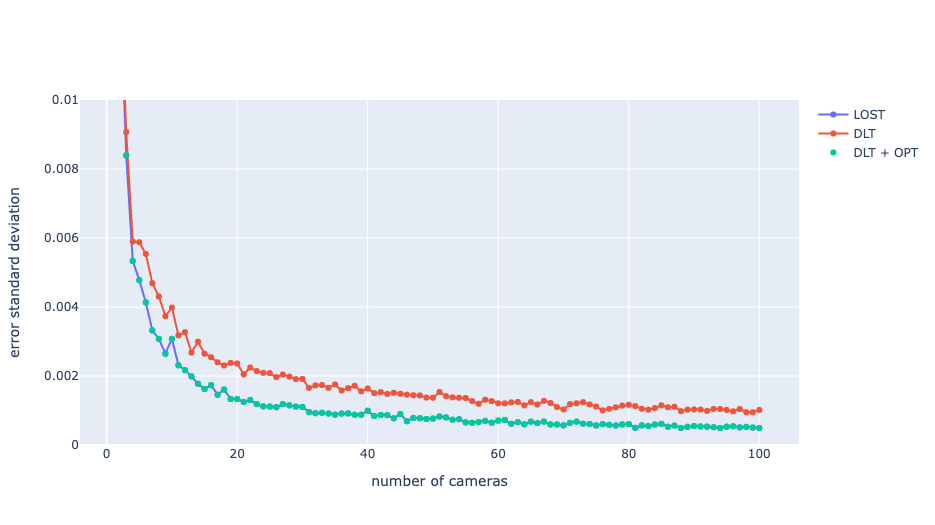
Fig 1: Error standard deviation for different triangulation methods as a function of number of cameras, with 100 trials for each camera configuration.
The latency of LOST is also comparable to DLT and is much lesser than that of iterative optimization. The mean latencies for these methods as a function of the number of cameras are plotted in Fig 2. The latency of iterative optimization increases more rapidly with an increase in the number of camera measurements.
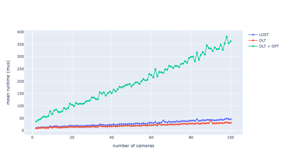
Fig 2: Mean runtime of different triangulation methods as a function of number of cameras.
There are two key conclusions from these numerical experiments. First, LOST provides identical triangulation performance (i.e., identical errors) as the iterative nonlinear least squares (DLT+OPT) but at a fraction of the computational cost. There seems to be a strong case for using LOST instead of the conventional iterative methods in most situations - especially when runtime is important. Second, there are certainly some cases (such as this one) where using optimal triangulation provides substantial performance benefits when compared to the DLT.
When does using optimal triangulation make the most difference?
Is optimal triangulation always better than DLT? There are two cases when it can provide much better results than DLT:
- The 3D point is at significantly different ranges from each camera that observes it. Since the covariance of the estimate increases with its range from the camera, optimal triangulation weighs measurements from closer cameras more than those from farther cameras. This can also be seen in (12): the weights of each measurement are inversely proportional to the $\rho_i$. The optimal estimates are therefore closer to the measurements from closer cameras.
- When different measurements have different 2D noise models. This can happen if the cameras observing these measurements are of different quality, or the measurement noise is non-uniformly distributed across the image (more on the edges and lesser at the center, for instance).
In other cases, the results from DLT and optimal triangulation are unlikely to be very different. For highly runtime-constrained applications that encounter the above scenarios, using LOST instead of results from DLT can reduce estimation errors.
References
- “Absolute Triangulation Algorithms for Space Exploration”, Sébastien Henry, John Christian, Journal of Guidance, Control, and Dynamics 2023 46:1, Pages 21-46. Arxiv version Aug ‘22
- “Triangulation”, Richard Hartley, Peter Sturm, Computer Vision and Image Understanding, November 1997, Volume 68, Issue 2, Pages 146-157