LQR Control Using Factor Graphs
GTSAM Posts
Authors: Gerry Chen, Yetong Zhang, and Frank Dellaert
Introduction
In this post we explain how optimal control problems can be formulated as factor graphs and solved by performing variable elimination on the factor graph.
Specifically, we will show the factor graph formulation and solution for the Linear Quadratic Regulator (LQR). LQR is a state feedback controller which derives the optimal gains for a linear system with quadratic costs on control effort and state error.
We consider the finite-horizon, discrete LQR problem. The task is to find the optimal controls $u_k$ at time instances $t_k$ so that a total cost is minimized. Note that we will later see the optimal controls can be represented in the form $u^*_k = K_kx_k$ for some optimal gain matrices $K_k$. The LQR problem can be represented as a constrained optimization problem where the costs of control and state error are represented by the minimization objective \eqref{eq:cost}, and the system dynamics are represented by the constraints \eqref{eq:dyn_model}.
\[ \begin{equation} \argmin\limits_{u_{1\sim N}} ~~x_N^T Q x_N + \sum\limits_{k=1}^{N-1} x_k^T Q x_k + u_k^T R u_k \label{eq:cost} \end{equation}\] \[ \begin{equation} s.t. ~~ x_{k+1}=Ax_k+Bu_k ~~\text{for } k=1 \text{ to } N-1 \label{eq:dyn_model} \end{equation} \]
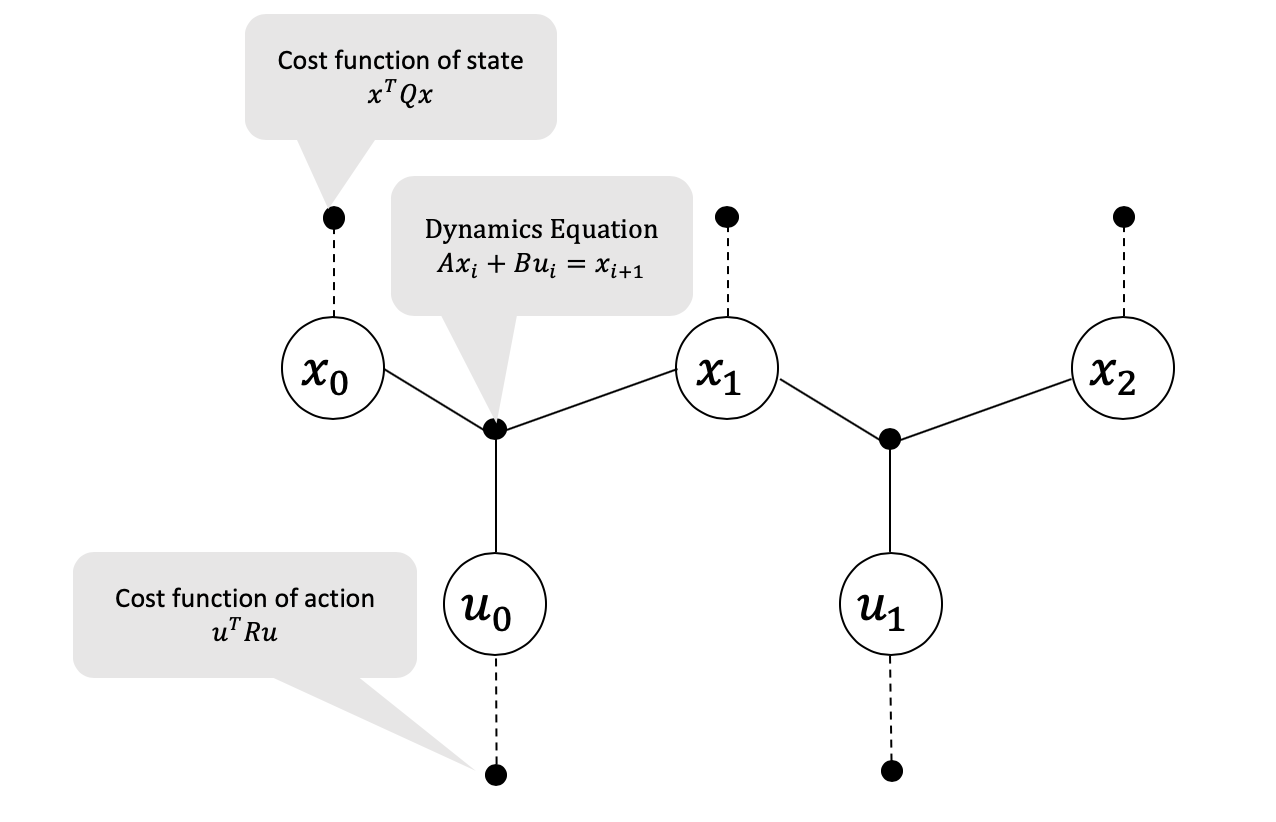
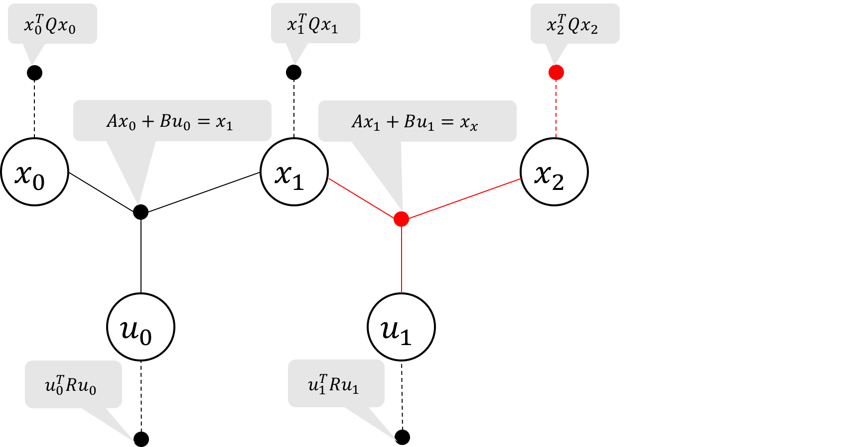
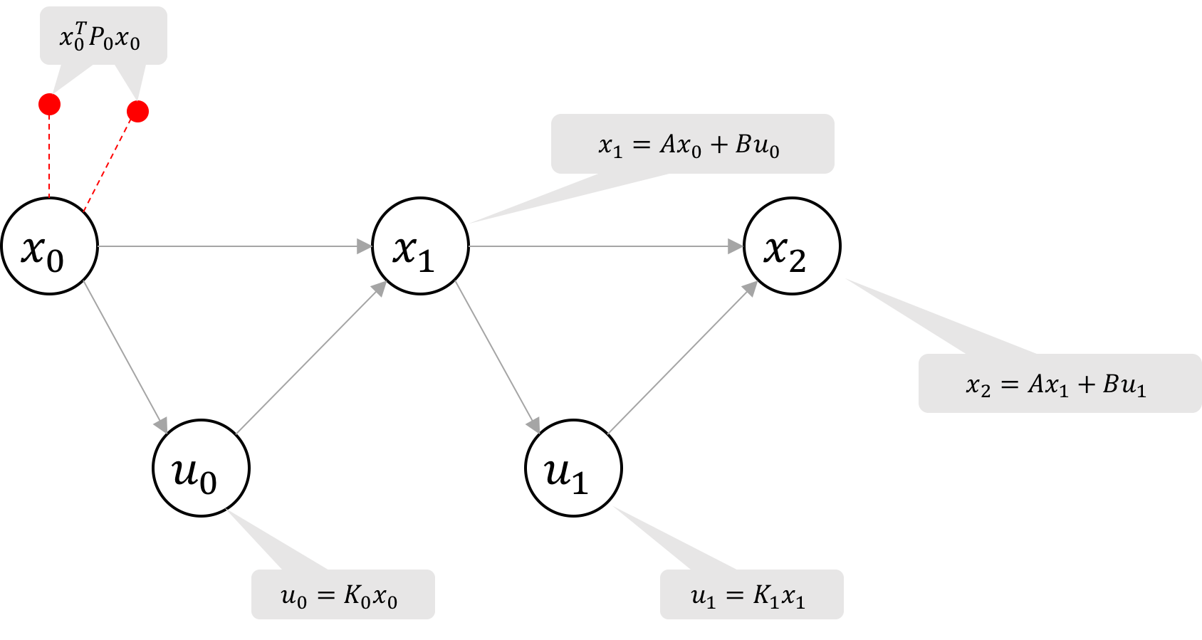
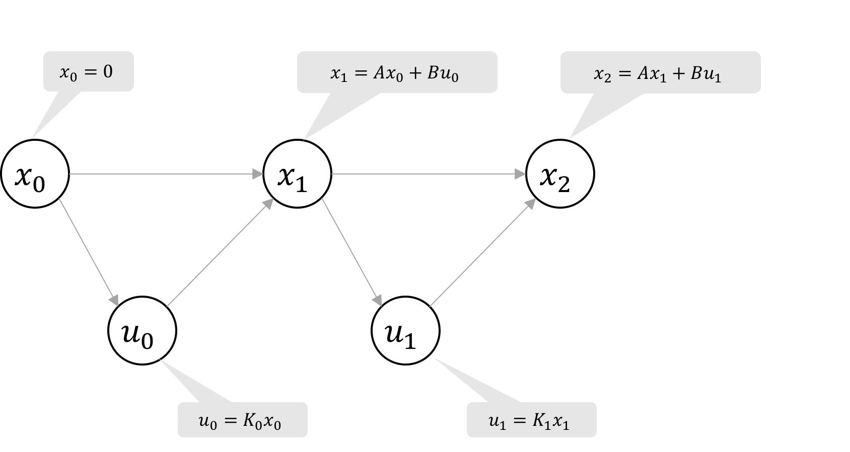
We can visualize the objective function and constraints in the form of a factor graph as shown in Figure 1. This is a simple Markov chain, with the oldest states and controls on the left, and the newest states and controls on the right. The ternary factors represent the dynamics model constraints and the unary factors represent the state and control costs we seek to minimize via least-squares.
Variable Elimination
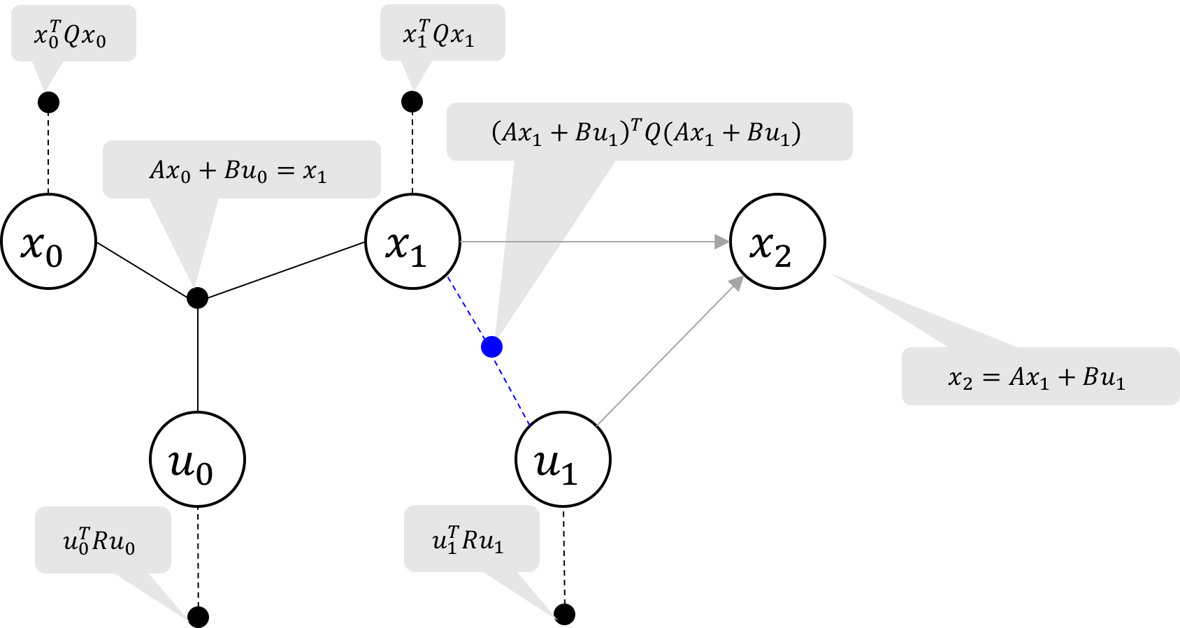
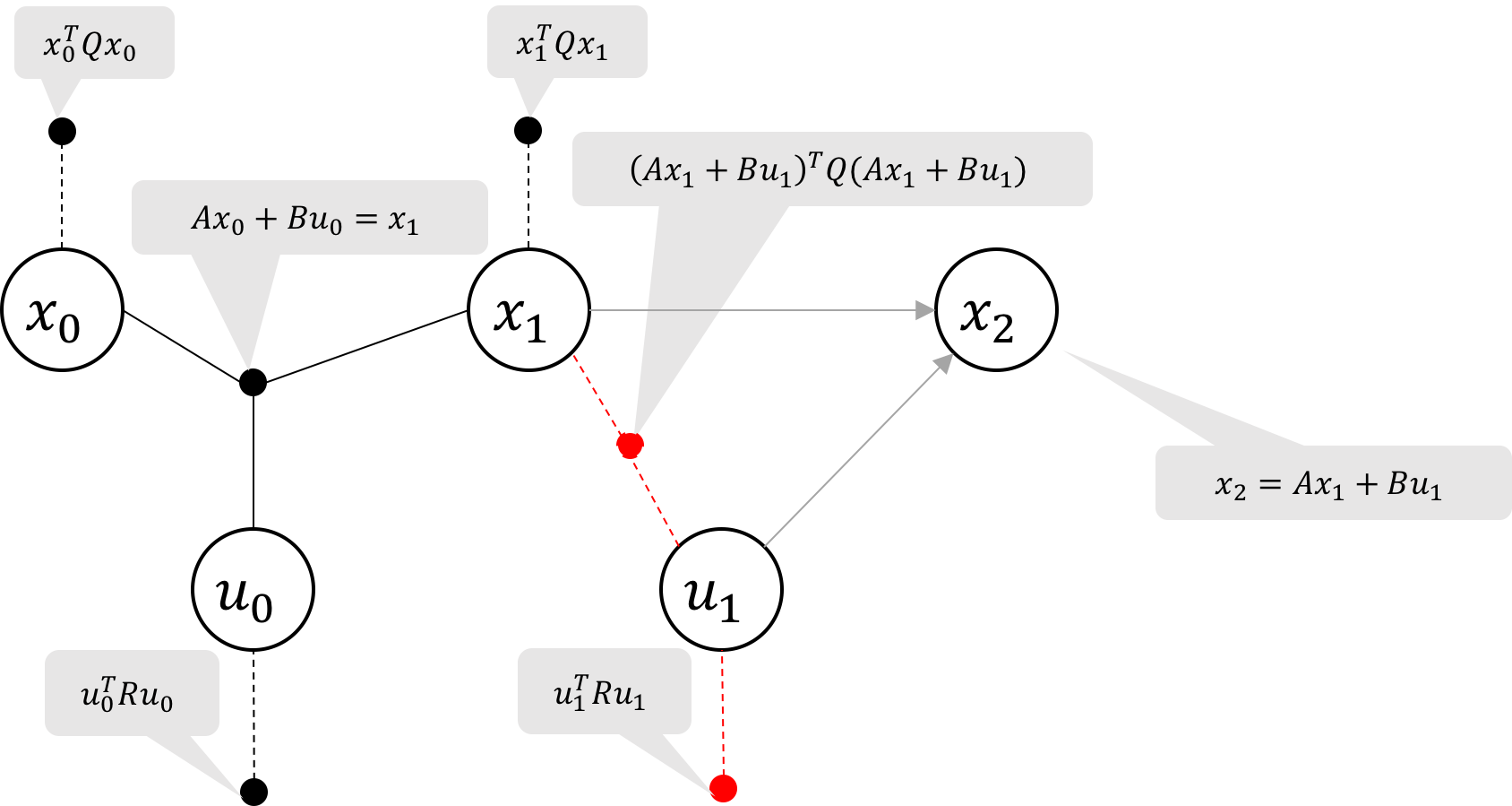
To optimize the factor graph, which represents minimizing the least squares objectives above, we can simply eliminate the factors from right to left. In this section we demonstrate the variable elimination graphically and algebraically, but the matrix elimination is also provided in the Appendix.
Intuition
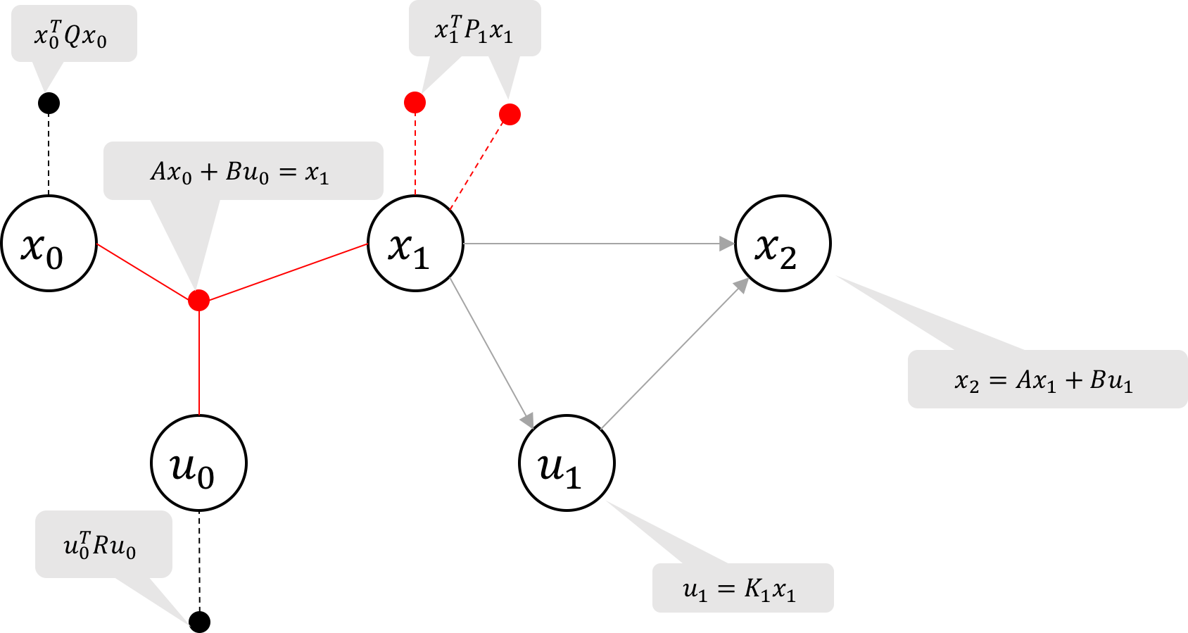
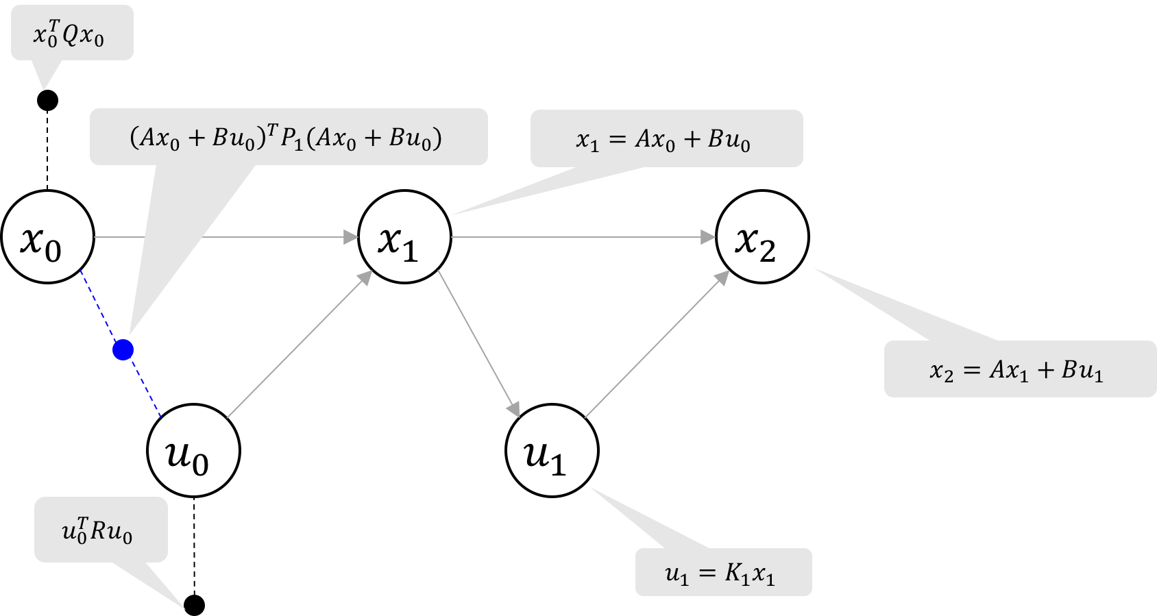
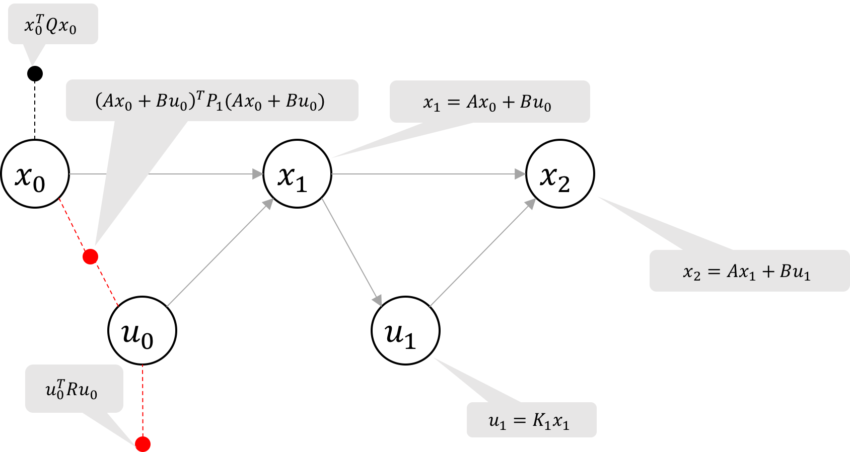
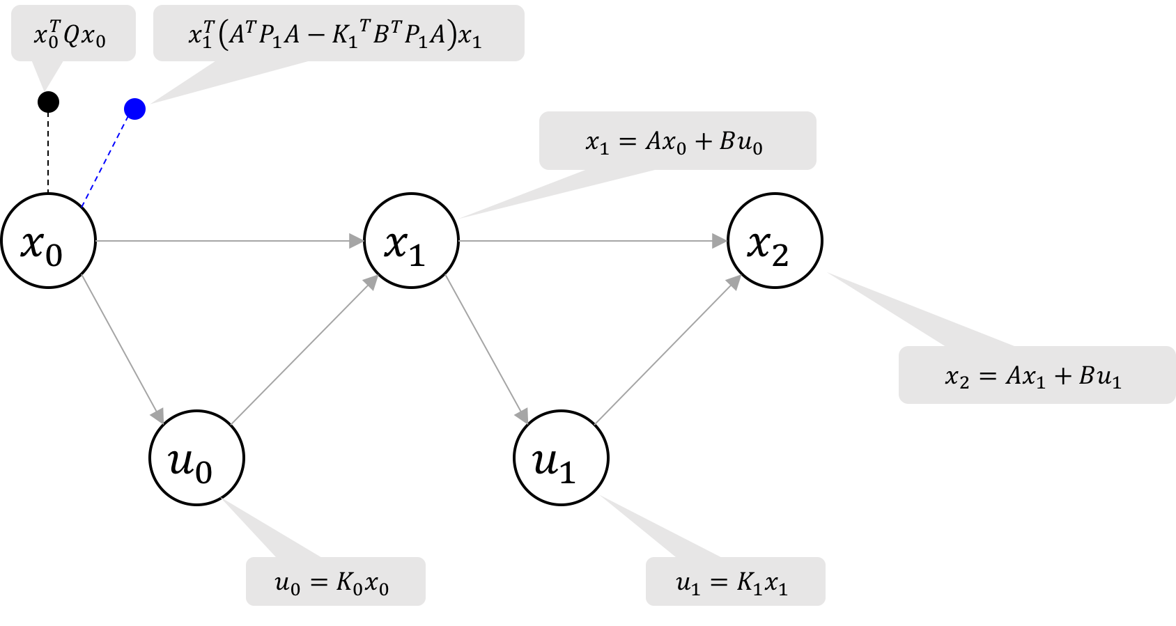
We introduce the cost-to-go (also known as return cost, optimal state value function, or simply value function) as $V_k(x) \coloneqq x^TP_kx$ which intuitively represents the total cost that will be accrued from here on out, assuming optimal control.
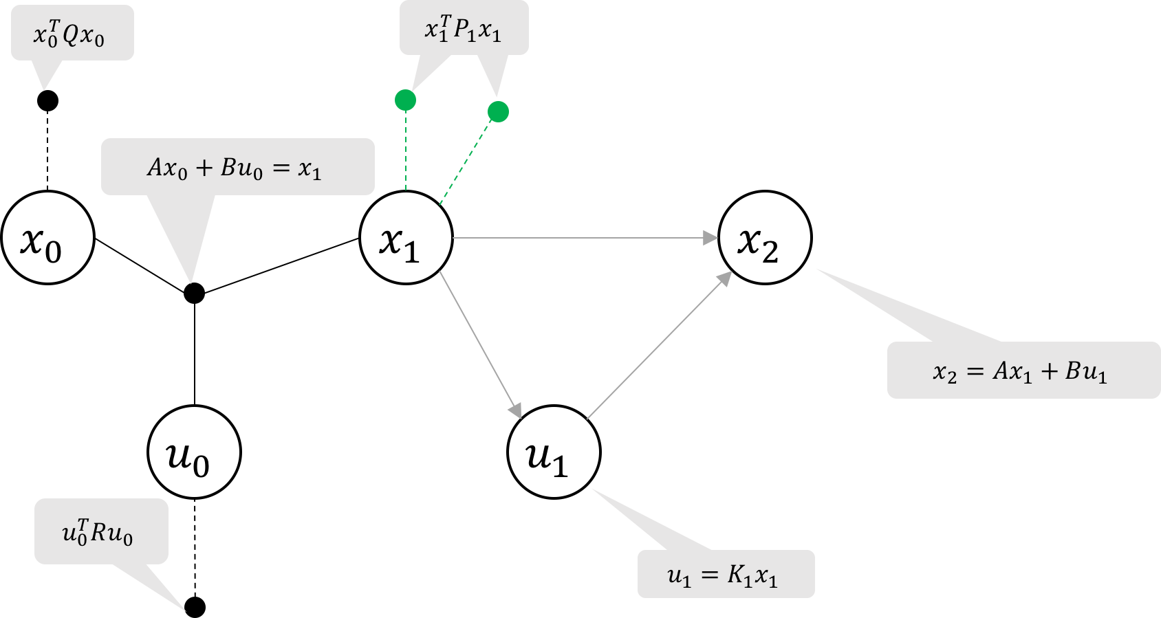
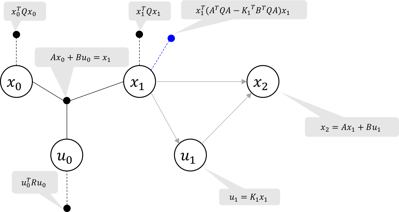
In our factor graph representation, it is becomes obvious that $V_k(x)$ corresponds to the total cost at and after the state $x_k$ assuming optimal control because we eliminate variables backwards in time with the objective of minimizing cost. Eliminating a state just re-expresses the future cost in terms of prior states/controls. Each time we eliminate a control, $u$, the future cost is recalculated assuming optimal control (i.e. $\phi_4(x) = \phi_3(x, u^*)$).
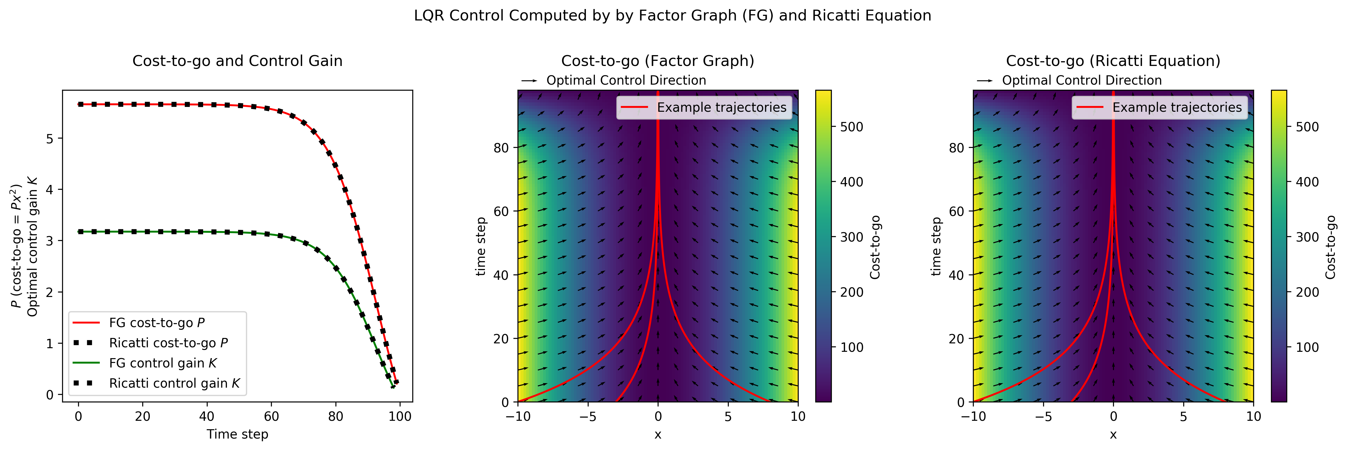
This “cost-to-go” is depicted as a heatmap in Figure 5. The heat maps depict the $V_k$ showing that the cost is high when $x$ is far from 0, but also showing that after iterating sufficient far backwards in time, $V_k(x)$ begins to converge. That is to say, the $V_0(x)$ is very similar for $N=30$ and $N=100$. Similarly, the leftmost plot of Figure 5 depicts $K_k$ and $P_k$ and shows that they (predictably) converge as well.
This convergence allows us to see that we can extend to the infinite horizon LQR problem (continued in the next section).
Equivalence to the Ricatti Equation
In traditional descriptions of discrete, finite-horizon LQR (i.e. Chow, Kirk, Stanford), the control law and cost function are given by
\[ u_k = K_kx_k \]
\begin{equation} K_k = -(R+B^TP_{k+1}B)^{-1}B^TP_{k+1}A \label{eq:control_update_k_ricatti} \end{equation}
\begin{equation} P_k = Q+A^TP_{k+1}A - K_k^TB^TP_{k+1}A \label{eq:cost_update_k_ricatti} \end{equation}
with $P_k$ commonly referred to as the solution to the dynamic Ricatti equation and $P_N=Q$ is the value of the Ricatti function at the final time step. \eqref{eq:control_update_k_ricatti} and \eqref{eq:cost_update_k_ricatti} correspond to the same results as we derived in \eqref{eq:control_update_k} and \eqref{eq:cost_update_k} respectively.
Recall that $P_0$ and $K_0$ appear to converge as the number of time steps grows. They will approach a stationary solution to the equations
\begin{align} K &= -(R+B^TPB)^{-1}B^TPA \nonumber \\ P &= Q+A^TPA - K^TB^TPA \nonumber \end{align}
as $N\to\infty$. This is the Discrete Algebraic Ricatti Equations (DARE) and $\lim_{N\to\infty}V_0(x)$ and $\lim_{N\to\infty}K_0$ are the cost-to-go and optimal control gain respectively for the infinite horizon LQR problem. Indeed, one way to calculate the solution to the DARE is to iterate on the dynamic Ricatti equation.
Implementation using GTSAM
**Edit (Apr 17, 2021): Code updated to new Python wrapper as of GTSAM 4.1.0.
You can view an example Jupyter notebook on google colab or download the modules/examples that you can use in your projects to:
- Calculate the closed loop gain matrix, K, using GTSAM
- Calculate the “cost-to-go” matrix, P (which is equivalent to the solutions to the dynamic Ricatti equation), using GTSAM
- Calculate the LQR solution for a non-zero, non-constant goal position, using GTSAM
- Visualize the cost-to-go and how it relates to factor graphs and the Ricatti equation
- and more!
A brief example of the open-loop finite horizon LQR problem using factor graphs is shown below:
def solve_lqr(A, B, Q, R, X0=np.array([0., 0.]), num_time_steps=500):
    '''Solves a discrete, finite horizon LQR problem given system dynamics in
    state space representation.
    Arguments:
        A, B: nxn state transition matrix and nxp control input matrix
        Q, R: nxn state cost matrix and pxp control cost matrix
        X0: initial state (n-vector)
        num_time_steps: number of time steps, T
    Returns:
        x_sol, u_sol: Txn array of states and Txp array of controls
    '''
    n = np.size(A, 0)
    p = np.size(B, 1)

    # noise models
    prior_noise = gtsam.noiseModel.Constrained.All(n)
    dynamics_noise = gtsam.noiseModel.Constrained.All(n)
    q_noise = gtsam.noiseModel.Gaussian.Information(Q)
    r_noise = gtsam.noiseModel.Gaussian.Information(R)

    # Create an empty Gaussian factor graph
    graph = gtsam.GaussianFactorGraph()

    # Create the keys corresponding to unknown variables in the factor graph
    X = []
    U = []
    for k in range(num_time_steps):
        X.append(gtsam.symbol('x', k))
        U.append(gtsam.symbol('u', k))

    # set initial state as prior
    graph.add(X[0], np.eye(n), X0, prior_noise)

    # Add dynamics constraint as ternary factor
    #   A.x1 + B.u1 - I.x2 = 0
    for k in range(num_time_steps-1):
        graph.add(X[k], A, U[k], B, X[k+1], -np.eye(n),
                  np.zeros((n)), dynamics_noise)

    # Add cost functions as unary factors
    for x in X:
        graph.add(x, np.eye(n), np.zeros(n), q_noise)
    for u in U:
        graph.add(u, np.eye(p), np.zeros(p), r_noise)

    # Solve
    result = graph.optimize()
    x_sol = np.zeros((num_time_steps, n))
    u_sol = np.zeros((num_time_steps, p))
    for k in range(num_time_steps):
        x_sol[k, :] = result.at(X[k])
        u_sol[k] = result.at(U[k])

    return x_sol, u_sol
Future Work
The factor graph (Figure 1) for our finite horizon discrete LQR problem can be readily extended to LQG, iLQR, DDP, and reinforcement learning using non-deterministic dynamics factors, nonlinear factors, discrete factor graphs, and other features of GTSAM (stay tuned for future posts).
Appendix
Least Squares Implementation in GTSAM
GTSAM can be specified to use either of two methods for solving the least squares problems that appear in eliminating factor graphs: Cholesky Factorization or QR Factorization. Both arrive at the same result, but we will take a look at QR since it more immediately illustrates the elimination algorithm at work.
QR Factorization
\( \begin{array}{cc} \text{NM} & \text{Elimination Matrix} \\ \left[ \begin{array}{c} \vphantom{Q^{1/2} | } I\\ \vphantom{I | } 0\\ \vphantom{R^{1/2} | } I\\ \vphantom{Q^{1/2} | } I\\ \vphantom{-A | } 0\\ \vphantom{R^{1/2} | } I\\ \vphantom{Q^{1/2} | } I \end{array} \right] & \left[ \begin{array}{ccccc|c} Q^{1/2} & & & & & 0\\ I & -B & -A & & & 0\\ & R^{1/2} & & & & 0\\ & & Q^{1/2}& & & 0\\ & & I & -B & -A & 0\\ & & & R^{1/2}& & 0\\ & & & & Q^{1/2}& 0 \end{array} \right] \end{array} \)
\( \begin{array}{cc} \text{NM} & \text{Elimination Matrix} \\ \begin{bmatrix} \vphantom{Q^{1/2} | } I\\ \vphantom{I | } 0\\ \vphantom{R^{1/2} | } I\\ \vphantom{Q^{1/2} | } I\\ \vphantom{I | } 0\\ \vphantom{R^{1/2} | } I\\ \vphantom{Q^{1/2} | } I \end{bmatrix} & \left[ \begin{array}{ccccc|c} \color{red} {Q^{1/2}} & & & & & 0\\ \color{red} I & \color{red} {-B} & \color{red} {-A} & & & 0\\ & R^{1/2} & & & & 0\\ & & Q^{1/2}& & & 0\\ & & I & -B & -A & 0\\ & & & R^{1/2}& & 0\\ & & & & Q^{1/2}& 0 \end{array} \right] \end{array} \)
\( \begin{array}{cc} \text{NM} & \text{Elimination Matrix} \\ \begin{bmatrix} \vphantom{I | } 0\\ \vphantom{Q^{1/2} | } I\\ \vphantom{R^{1/2} | } I\\ \vphantom{Q^{1/2} | } I\\ \vphantom{I | } 0\\ \vphantom{R^{1/2} | } I\\ \vphantom{Q^{1/2} | } I\\ \end{bmatrix} & \left[ \begin{array}{c:cccc|c} I & -B & -A & & & 0\\ \hdashline & \color{blue} {Q^{1/2}B} & \color{blue} {Q^{1/2}A} & & & 0\\ & R^{1/2} & & & & 0\\ & & Q^{1/2}& & & 0\\ & & I & -B & -A & 0\\ & & & R^{1/2}& & 0\\ & & & & Q^{1/2}& 0 \end{array} \right] \end{array} \)
\( \begin{array}{cc} \text{NM} & \text{Elimination Matrix} \\ \begin{bmatrix} \vphantom{I | } 0\\ \vphantom{Q^{1/2} | } I\\ \vphantom{R^{1/2} | } I\\ \vphantom{Q^{1/2} | } I\\ \vphantom{I | } 0\\ \vphantom{R^{1/2} | } I\\ \vphantom{Q^{1/2} | } I\\ \end{bmatrix} & \left[ \begin{array}{c:cccc|c} I & -B & -A & & & 0\\ \hdashline & \color{red} {Q^{1/2}B} & \color{red} {Q^{1/2}A} & & & 0\\ & \color{red} {R^{1/2}} & & & & 0\\ & & {Q^{1/2}} & & & 0\\ & & I & -B & -A & 0\\ & & & R^{1/2}& & 0\\ & & & & Q^{1/2}& 0 \end{array} \right] \end{array} \)
\( \begin{array}{cc} \text{NM} & \text{Elimination Matrix} \\ \begin{bmatrix} \vphantom{I | } 0\\ \vphantom{D_1^{1/2} | } I\\ \vphantom{(P_1-Q)^{1/2} | } I\\ \vphantom{Q^{1/2} | } I\\ \vphantom{I | } 0\\ \vphantom{R^{1/2} | } I\\ \vphantom{Q^{1/2} | } I\\ \end{bmatrix} & \left[ \begin{array}{cc:ccc|c} I & -B & -A & & & 0\\ & D_1^{1/2} & -D_1^{1/2}K_1 & & & 0\\ \hdashline & & \color{blue} {(P_1-Q)^{1/2}} & & & 0\\ & & Q^{1/2} & & & 0\\ & & I & -B & -A & 0\\ & & & R^{1/2}& & 0\\ & & & & Q^{1/2}& 0 \end{array} \right] \end{array} \)
\( \begin{array}{cc} \text{NM} & \text{Elimination Matrix} \\ \begin{bmatrix} \vphantom{I | } 0\\ \vphantom{D_1^{1/2} | } I\\ \vphantom{(P_1-Q)^{1/2} | } I\\ \vphantom{Q^{1/2} | } I\\ \vphantom{I | } 0\\ \vphantom{R^{1/2} | } I\\ \vphantom{Q^{1/2} | } I\\ \end{bmatrix} & \left[ \begin{array}{cc:ccc|c} I & -B & -A & & & 0\\ & D_1^{1/2} & -D_1^{1/2}K_1 & & & 0\\ \hdashline & & \color{red} {(P_1-Q)^{1/2}} & & & 0\\ & & \color{red} {Q^{1/2}} & & & 0\\ & & \color{red} I & \color{red} {-B} & \color{red} {-A} & 0\\ & & & R^{1/2}& & 0\\ & & & & Q^{1/2}& 0 \end{array} \right] \end{array} \)
\( \begin{array}{cc} \text{NM} & \text{Elimination Matrix} \\ \begin{bmatrix} \vphantom{I | } 0\\ \vphantom{D_1^{1/2}K_1 | } I\\ \vphantom{I | } 0\\ \vphantom{D_0^{1/2} | } I\\ \vphantom{P^{1/2} | } I\\ \vphantom{Q^{1/2} | } I\\ \end{bmatrix} & \left[ \begin{array}{ccc:cc|c} I & -B & -A & & & 0\\ & D_1^{1/2} & -D_1^{1/2}K_1& & & 0\\ & & I & -B & -A & 0\\ \hdashline & & &\color{blue} {P_1^{1/2}B} & \color{blue} {P_1^{1/2}A} & 0\\ & & & R^{1/2}& & 0\\ & & & & Q^{1/2}& 0 \end{array} \right] \end{array} \)
\( \begin{array}{cc} \text{NM} & \text{Elimination Matrix} \\ \begin{bmatrix} \vphantom{I | } 0\\ \vphantom{D_1^{1/2}K_1 | } I\\ \vphantom{I | } 0\\ \vphantom{D_0^{1/2} | } I\\ \vphantom{P^{1/2} | } I\\ \vphantom{Q^{1/2} | } I\\ \end{bmatrix} & \left[ \begin{array}{ccc:cc|c} I & -B & -A & & & 0\\ & D_1^{1/2} & -D_1^{1/2}K_1& & & 0\\ & & I & -B & -A & 0\\ \hdashline & & &\color{red} {P_1^{1/2}B} &\color{red} {P_1^{1/2}A} & 0\\ & & &\color{red} {R^{1/2}} & & 0\\ & & & & Q^{1/2} & 0 \end{array} \right] \end{array} \)
\( \begin{array}{cc} \text{NM} & \text{Elimination Matrix} \\ \begin{bmatrix} \vphantom{I | } 0\\ \vphantom{D_1^{1/2}K_1 | } I\\ \vphantom{I | } 0\\ \vphantom{D_0^{1/2} | } I\\ \vphantom{(P_0-Q)^{1/2} | } I\\ \vphantom{P^{1/2} | } I\\ \end{bmatrix} & \left[ \begin{array}{cccc:c|c} I & -B & -A & & & 0\\ & D_1^{1/2} & -D_1^{1/2}K_1 & & & 0\\ & & I & -B & -A & 0\\ & & & D_0^{1/2} & -D_0^{1/2}K_0 & 0\\ \hdashline & & & & \color{blue} {(P_0-Q)^{1/2}} & 0\\ & & & & Q^{1/2} & 0\\ \end{array} \right] \end{array} \)
\( \begin{array}{cc} \text{NM} & \text{Elimination Matrix} \\ \begin{bmatrix} \vphantom{I | } 0\\ \vphantom{D_1^{1/2}K_1 | } I\\ \vphantom{I | } 0\\ \vphantom{D_0^{1/2} | } I\\ \vphantom{(P_0-Q)^{1/2} | } I\\ \vphantom{P^{1/2} | } I\\ \end{bmatrix} & \left[ \begin{array}{cccc:c|c} I & -B & -A & & & 0\\ & D_1^{1/2} & -D_1^{1/2}K_1 & & & 0\\ & & I & -B & -A & 0\\ & & & D_0^{1/2} & -D_0^{1/2}K_0 & 0\\ \hdashline & & & & \color{red} {(P_0-Q)^{1/2}} & 0\\ & & & & \color{red} {Q^{1/2}} & 0\\ \end{array} \right] \end{array} \)
\( \begin{array}{cc} \text{NM} & \text{Elimination Matrix} \\ \begin{bmatrix} \vphantom{I | } 0\\ \vphantom{D_1^{1/2}K_1 | } I\\ \vphantom{I | } 0\\ \vphantom{D_0^{1/2} | } I\\ \vphantom{P_0^{1/2} | } I\\ \end{bmatrix} & \left[ \begin{array}{cccc:c|c} I & -B & -A & & & 0\\ & D_1^{1/2} & -D_1^{1/2}K_1 & & & 0\\ & & I & -B & -A & 0\\ & & & D_0^{1/2} & -D_0^{1/2}K_0 & 0\\ \hdashline & & & & \color{blue} {P_0^{1/2}} & 0\\ \end{array} \right] \end{array} \)
| where | $P_{k}$ | $=$ | $Q + A^TP_{k+1}A - K_k^TB^TP_{k+1}A$ | ($P_2=Q$) |
|---|---|---|---|---|
| $D_{k}$ | $=$ | $R + B^TP_{k+1}B$ | ||
| $K_k$ | $=$ | $-D_{k}^{-1/2}(R + B^TP_{k+1}B)^{-T/2}B^TP_{k+1}A$ | ||
| $=$ | $-(R + B^TP_{k+1}B)^{-1}B^TP_{k+1}A$ |
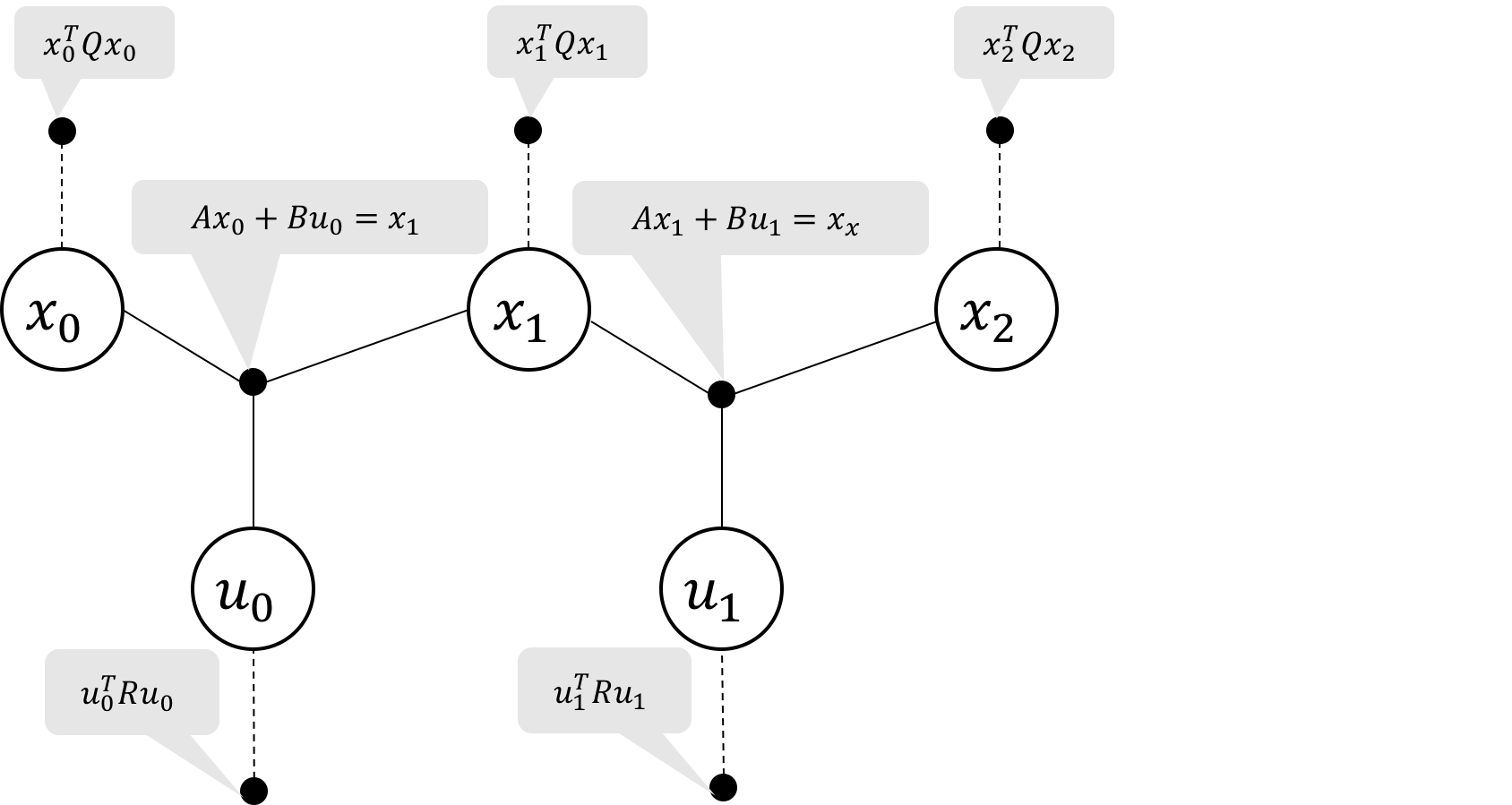
The factorization process is illustrated in Figure 6 for a 3-time step factor graph, where the noise matrices and elimination matrices are shown with the corresponding states of the graph. The noise matrix (NM) is $0$ for a hard constraint and $I$ for a minimization objective. The elimination matrix is formatted as an augmented matrix $[A|b]$ for the linear least squares problem $\argmin\limits_x||Ax-b||_2^2$ with ${x=[x_2;u_1;x_1;u_0;x_0]}$ is the vertical concatenation of all state and control vectors. The recursive expressions for $P$, $D$, and $K$ when eliminating control variables (i.e. $u_1$ in Figure 6e) are derived from block QR Factorization.
Note that all $b_i=0$ in the augmented matrix for the LQR problem of finding minimal control to reach state $0$, but simply changing values of $b_i$ intuitively extends GTSAM to solve LQR problems whose objectives are to reach different states or even follow trajectories.