Look Ma, No RANSAC
GTSAM Posts
Author: Varun Agrawal
Website: varunagrawal.github.io
(Psst, be sure to clone/download GTSAM 4.0.2 which resolves a bug in the Huber model discussed below, for correct weight behavior)
Introduction
Robust error models are powerful tools for supplementing parameter estimation algorithms with the added capabilities of modeling outliers. Parameter estimation is a fundamental tool used in many fields, especially in perception and robotics, and thus performing robust parameter estimation across a wide range of applications and scenarios is crucial to strong performance for many applications. This necessitates the need to manage outliers in our measurements, and robust error models provide us the means to do so. Robust error models are amenable to easy plug-and-play use in pre-existing optimization frameworks, requiring minimal changes to existing pipelines.
Using robust error models can even obviate the need for more complex, non-deterministic algorithms such as Random Sample Consensus (a.k.a. RANSAC), a fundamental tool for parameter estimation in many a roboticist’s toolbox for years. While RANSAC has proven to work well in practice, it might need a high number of runs to converge to a good solution. Robust error models are conceptually easy and intuitive and can be used by themselves or in conjunction with RANSAC.
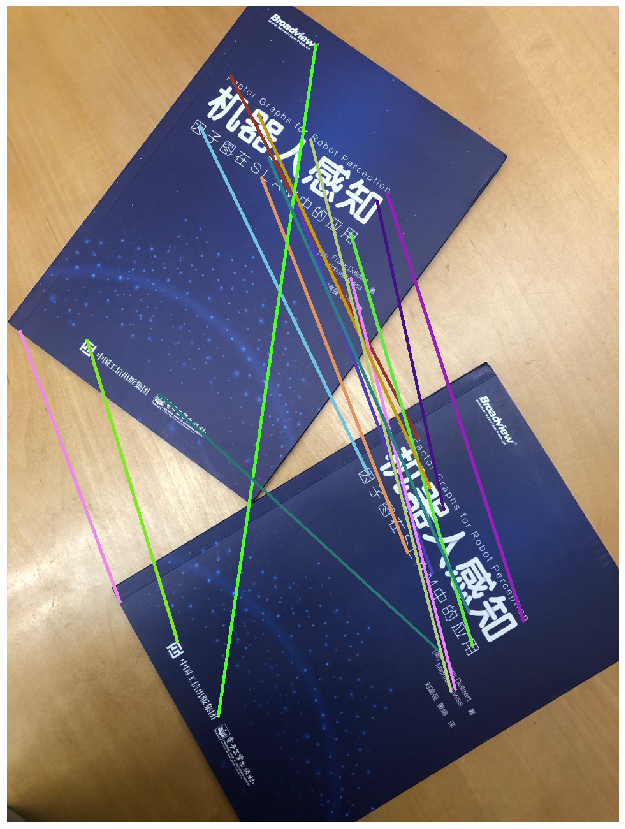
In this blog post, we demonstrate the capabilities of robust error models which downweigh outliers to provide better estimates of the parameters of interest. To illustrate the benefits of robust error models, take a look at Figure 1. We show two books next to each other, transformed by an $SE(2)$ transform, with some manually labeled point matches between the two books. We have added some outliers to more realistically model the problem. As we will see later in the post, the estimates from RANSAC and a robust estimation procedure are quite similar, even though the ratio of inliers to outliers is $2:1$.
Parameter Estimation - A Short Tutorial
We begin by reviewing techniques for parameter estimation as outlined by the tutorial by Zhengyou Zhang, as applied to our $SE(2)$. Given some matches ${(s,s’)}$ between the two images, we want to estimate the the $SE(2)$ parameters $\theta$ that transform a feature $s$ in the first image to a feature $s’$ in the second image:
\[ s’ = f(\theta ; s) \]
Of course, this generalizes to other transformations, including 3D-2D problems. This is a ubiquitous problem seen in multiple domains of perception and robotics and is referred to as parameter estimation.
A standard framework to estimate the parameters is via the Least-Squares formulation. We usually have many more observations than we have parameters, i.e., the problem is now overdetermined. To handle this, we minimize the sum of square residuals $f(\theta ; s_i) - s’_i$, for $i\in1\ldots N$:
\[ E_{LS}(\theta) = \sum_i \vert\vert f(\theta ; s_i) - s’_i \vert\vert^2 \]
which we refer to as the cost function or the objective function. In the case of $SE(2)$ the parameters $\theta$ should be some parameterization of a transformation matrix, having three degrees of freedom (DOF). A simple way to accomplish this is to have $\theta=(x,y,\alpha)$.
Our measurement functions are generally non-linear, and hence we need to linearize the measurement function around an estimate of $\theta$. GTSAM will iteratively do so via optimization procedures such as Gauss-Newton, Levenberg-Marquardt, or Dogleg. Linearization is done via the Taylor expansion around a linearization point $\theta_0$:
\[ f(\theta + \Delta\theta; s) = f(\theta; s) + J(\theta; s)\Delta\theta \]
This gives us the following linearized least squares objective function:
\[ E_{LS, \theta_0} = \sum_i \vert\vert f(\theta; s_i) + J(\theta; s_i)\Delta\theta - s_i’ \vert\vert^2 \]
Since the above is now linear in $\Delta\theta$, GTSAM can solve it using either sparse Cholesky or QR factorization.
Robust Error Models
We have derived the basic parameter optimization approach in the previous section and seen how the choice of the optimization function affects the optimality of our solution. However, another aspect we need to take into account is the effect of outliers on our optimization and final parameter values.
By default, the optimization objectives outlined above try to model all measurements equally. This means that in the presence of outliers, the optimization process might give us parameter estimates that try to fit these outliers, sacrificing accuracy on the inliers. More formally, given the residual $r_i$ of the $i^{th}$ match, i.e. the difference between the $i^{th}$ observation and the fitted value, the standard least squares approach attempts to optimize the sum of all the squared residuals. This can lead to the estimated parameters being distorted due to the equal weighting of all data points. Surely, there must be a way for the objective to model inliers and outliers in a clever way based on the residual errors?
One way to tackle the presence of outliers is a family of models known as Robust Error Models or M-estimators. The M-estimators try to reduce the effect of outliers by replacing the squared residuals with a function of the residuals $\rho$ that weighs each residual term by some value:
\[ p = min \sum_i^n \rho(r_i) \]
To allow for optimization, we define $\rho$ to be a symmetric, positive-definite function, thus it has a unique minimum at zero, and is less increasing than square.
The benefit of this formulation is that we can now solve the above minimization objective as an Iteratively Reweighted Least Squares problem. The M-estimator of the parameter vector $p$ based on $\rho$ is the value of the parameters which solves
\[ \sum_i \psi(r_i)\frac{\delta r_i}{\delta p_j} = 0 \]
for $j = 1, …, m$ (recall that the maximum/minimum of a function is at the point its derivative is equal to zero). Above, $\psi(x) = \frac{\delta \rho(x)}{\delta x}$ is called the influence function, which we can use to define a weight function $w(x) = \frac{\psi{x}}{x}$ giving the original derivative as
\[ \sum_i w(r_i) r_i \frac{\delta r_i}{\delta p_j} = 0 \]
which is exactly the system of equations we obtain from iterated reweighted least squares.
In layman’s terms, the influence function $\psi(x)$ measures the influence of a data point on the value of the parameter estimate. This way, the estimated parameters are intelligent to outliers and only sensitive to inliers, since the are no longer susceptible to being significantly modified by a single match, thus making them robust.
M-estimator Constraints
While M-estimators provide us with significant benefits with respect to outlier modeling, they do come with some constraints which are required to enable their use in a wide variety of optimization problems.
- The influence function should be bounded.
- The robust estimator should be unique, i.e. it should have a unique minimum. This implies that the individual $\rho$-function is convex in variable p.
- The objective should have a gradient, even when the 2nd derivative is singular.
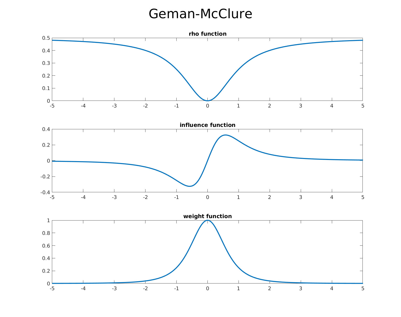
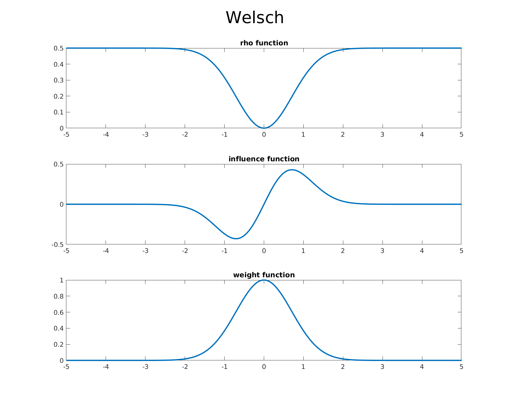
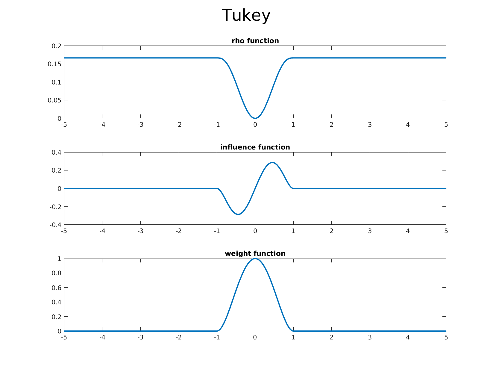
Common M-estimators
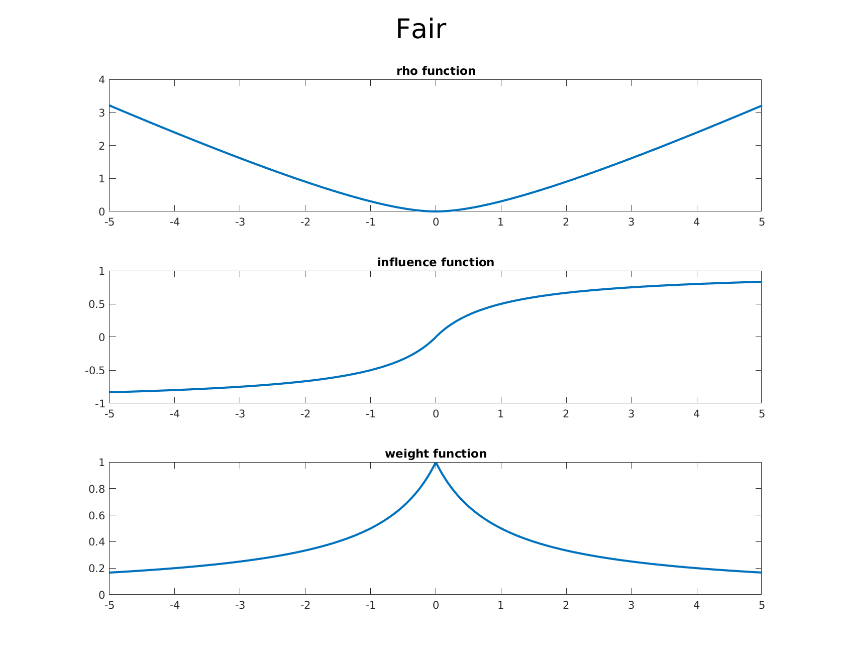
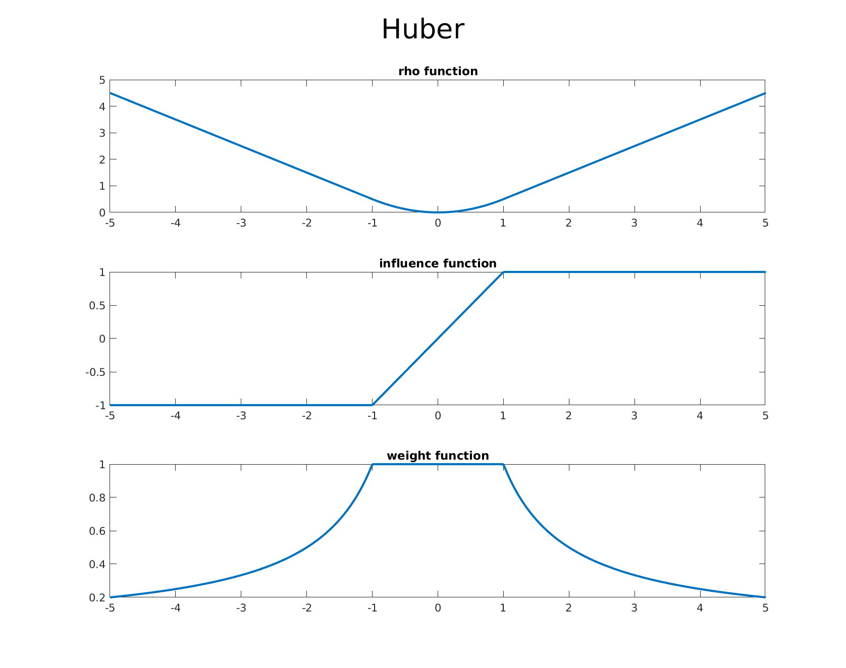
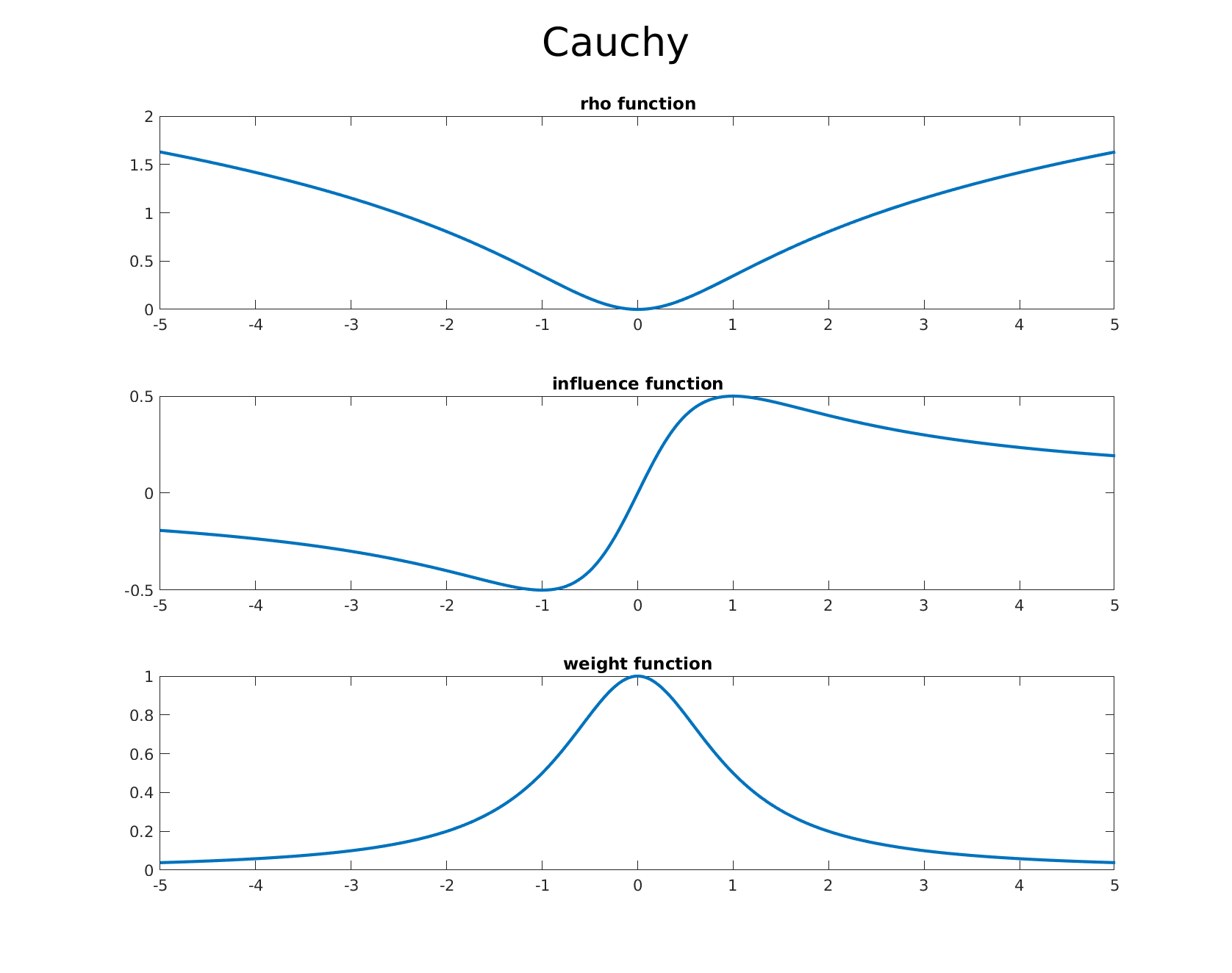
Below we list some of the common estimators from the literature and which are available out of the box in GTSAM. We also provide accompanying graphs of the corresponding $\rho$ function, the influence function, and the weight function in order, allowing one to visualize the differences and effects of each estimators influence function.
-
Fair
-
Huber
-
Cauchy
-
Geman-McClure
-
Welsch
-
Tukey
Example with Huber Noise Model
Now it’s time for the real deal. So far we’ve spoken about how great robust estimators are, and how they can be easily modeled in a least squares objective, but having a concrete example and application can really help illuminate these concepts and demonstrate the power of a robust error model. In this specific case we use the Huber M-estimator, though any other provided M-estimator can be used depending on the application or preference.
For our example application, the estimation of an $SE(2)$ transformation between two objects (a scenario commonly seen in PoseSLAM applications), we go back to our image of the two books from the introduction, which we have manually labeled with matches and outliers. A RANSAC estimate using the matches gives us the $SE(2)$ paramters (347.15593, 420.31040, 0.39645).
To begin, we apply a straightforward optimization process based on Factor Graphs. Using GTSAM, this can be achieved in a few lines of code. We show the core part of the example below, omitting the housekeeping and data loading for brevity.
// This is the value we wish to estimate
Pose2_ pose_expr(0);

// Set up initial values, and Factor Graph
Values initial;
ExpressionFactorGraph graph;

// provide an initial estimate which is pretty much random
initial.insert(0, Pose2(1, 1, 0.01));

// We assume the same noise model for all points (since it is the same camera)
auto measurementNoise = noiseModel::Isotropic::Sigma(2, 1.0);

// Now we add in the factors for the measurement matches.
// Matches is a vector of 4 tuples (index1, keypoint1, index2, keypoint2)
int index_i, index_j;
Point2 p, measurement;
for (vector<tuple<int, Point2, int, Point2>>::iterator it = matches.begin();
    it != matches.end(); ++it) {

    std::tie(index_i, measurement, index_j, p) = *it;

    Point2_ predicted = transformTo(pose_expr, p);

    // Add the Point2 expression variable, an initial estimate, and the measurement noise.
    graph.addExpressionFactor(predicted, measurement, measurementNoise);
}

// Optimize and print basic result
Values result = LevenbergMarquardtOptimizer(graph, initial).optimize();
result.print("Final Result:\n");
It is important to note that our initial estimate for the transform values is pretty arbitrary.
Running the above code give us the transform values (305.751, 520.127, 0.284743), which when compared to the RANSAC estimate doesn’t look so good.
Now how about we try using M-estimators via the built-in robust error models? This is a two line change as illustrated below:
// This is the value we wish to estimate
Pose2_ pose_expr(0);

// Set up initial values, and Factor Graph
Values initial;
ExpressionFactorGraph graph;

// provide an initial estimate which is pretty much random
initial.insert(0, Pose2(1, 1, 0.01));

// We assume the same noise model for all points (since it is the same camera)
auto measurementNoise = noiseModel::Isotropic::Sigma(2, 1.0);

/********* First change *********/
// We define our robust error model here, providing the default parameter value for the estimator.
auto huber = noiseModel::Robust::Create(noiseModel::mEstimator::Huber::Create(1.345), measurementNoise);

// Now we add in the factors for the measurement matches.
// Matches is a vector of 4 tuples (index1, keypoint1, index2, keypoint2)
int index_i, index_j;
Point2 p, measurement;
for (vector<tuple<int, Point2, int, Point2>>::iterator it = matches.begin();
    it != matches.end(); ++it) {

    std::tie(index_i, measurement, index_j, p) = *it;

    Point2_ predicted = transformTo(pose_expr, p);

    // Add the Point2 expression variable, an initial estimate, and the measurement noise.
    // The graph takes in factors with the robust error model.
    /********* Second change *********/
    graph.addExpressionFactor(predicted, measurement, huber);
}

// Optimize and print basic result
Values result = LevenbergMarquardtOptimizer(graph, initial).optimize();
result.print("Final Result:\n");
This version of the parameter estimation gives us the $SE(2)$ transform (363.76, 458.966, 0.392419). Quite close for only 15 total matches, especially considering 5 of the 10 were outliers! The estimates are expected to improve with more matches to further constrain the problem.
As an alternate example, we look at an induced $SE(2)$ transform and try to estimate it from scratch (no manual match labeling. Our source image is one of crayon boxes retrieved from the internet, since this image lends itself to good feature detection.

To model an $SE(2)$ transformation, we apply a perspective transform to the image. The transformation applied is (x, y, theta) = (4.711, 3.702, 0.13963). This gives us a ground truth value to compare our methods against. The transformed image can be seen below.

We run the standard pipeline of SIFT feature extraction and FLANN+KDTree based matching to obtain a set of matches. At this point we are ready to evaluate the different methods of estimating the transformation.
The vanilla version of the parameter estimation gives us (6.26294, -14.6573, 0.153888) which is pretty bad. However, the version with robust error models gives us (4.75419, 3.60199, 0.139674), which is a far better estimate when compared to the ground truth, despite the initial estimate for the transform being arbitrary. This makes it apparent that the use of robust estimators and subsequently robust error models is the way to go for use cases where outliers are a concern. Of course, providing better initial estimates will only improve the final estimate.
You may ask how does this compare to our dear old friend RANSAC? Using the OpenCV implementation of RANSAC, a similar pipeline gives use the following $SE(2)$ values: (4.77360, 3.69461, 0.13960).
We show, in order, the original image, its warped form, and the recovered image from the $SE(2)$ transformation estimation. The first image is from the ground truth transform, the second one is using RANSAC, the next one is using a vanilla parameter estimation approach, and the last one uses robust error models. As you can see, while the vanilla least-squares optimization result is poor compared to the ground truth, the RANSAC and the robust error model recover the transformation correctly, with the robust error model’s result being comparable to the RANSAC one.


Conclusion
In this post, we have seen the basics of parameter estimation, a ubiquitous mathematical framework for many perception and robotics problems, and we have seen how this framework is susceptible to perturbations from outliers which can throw off the final estimate. More importantly, we have seen how a simple tool called the Robust M-estimator can easily help us deal with these outliers and their effects. An example case for $SE(2)$ transform estimation demonstrates not only their ease of use with GTSAM, but also the efficacy of the solution generated, especially when compared to widely used alternatives such as RANSAC.
Furthermore, robust estimators are deterministic, ameliorating the need for the complexity that comes inherent with RANSAC. While RANSAC is a great tool, robust error models provide us with a solid alternative to be considered. With the benefits of speed, accuracy, and ease of use, robust error models make a strong case for their adoption for many related problems and we hope you will give them a shot the next time you use GTSAM.