Legged Robot Factors Part I
Author: Ross Hartley
email: m.ross.hartley@gmail.com
This is the first blog post in a series about using factor graphs for legged robot state estimation. It is meant to provide a high-level overview of what I call kinematic and contact factors and how they can be used in GTSAM. More details can be found in our conference papers:
- Hybrid Contact Preintegration for Visual-Inertial-Contact State Estimation Using Factor Graphs
- Legged Robot State-Estimation Through Combined Forward Kinematic and Preintegrated Contact Factors
It is assumed that the reader is already familiar with the terminology and theory behind factor graph based smoothing.
So, what makes legged robots different?
Factor graph methods have been widely successful for mobile robot state estimation and SLAM. A common application is the fusion of inertial data (from an IMU) with visual data (from camera and/or LiDAR sensors) to estimate the robot’s pose over time.
Although this approach is often demonstrated on wheeled and flying robots, identical techniques can be applied to their walking brethren. What makes legged robots different, however, is the presence of additional encoder and contact sensors. As I’ll show, these extra sensor measurements can be leveraged to improve state estimation results.
Sensors typically found on legged robots:
- Inertial Measurement Units (IMUs)
- Vision Sensors (cameras, LiDARs)
- Joint Encoders
- Contact Sensors
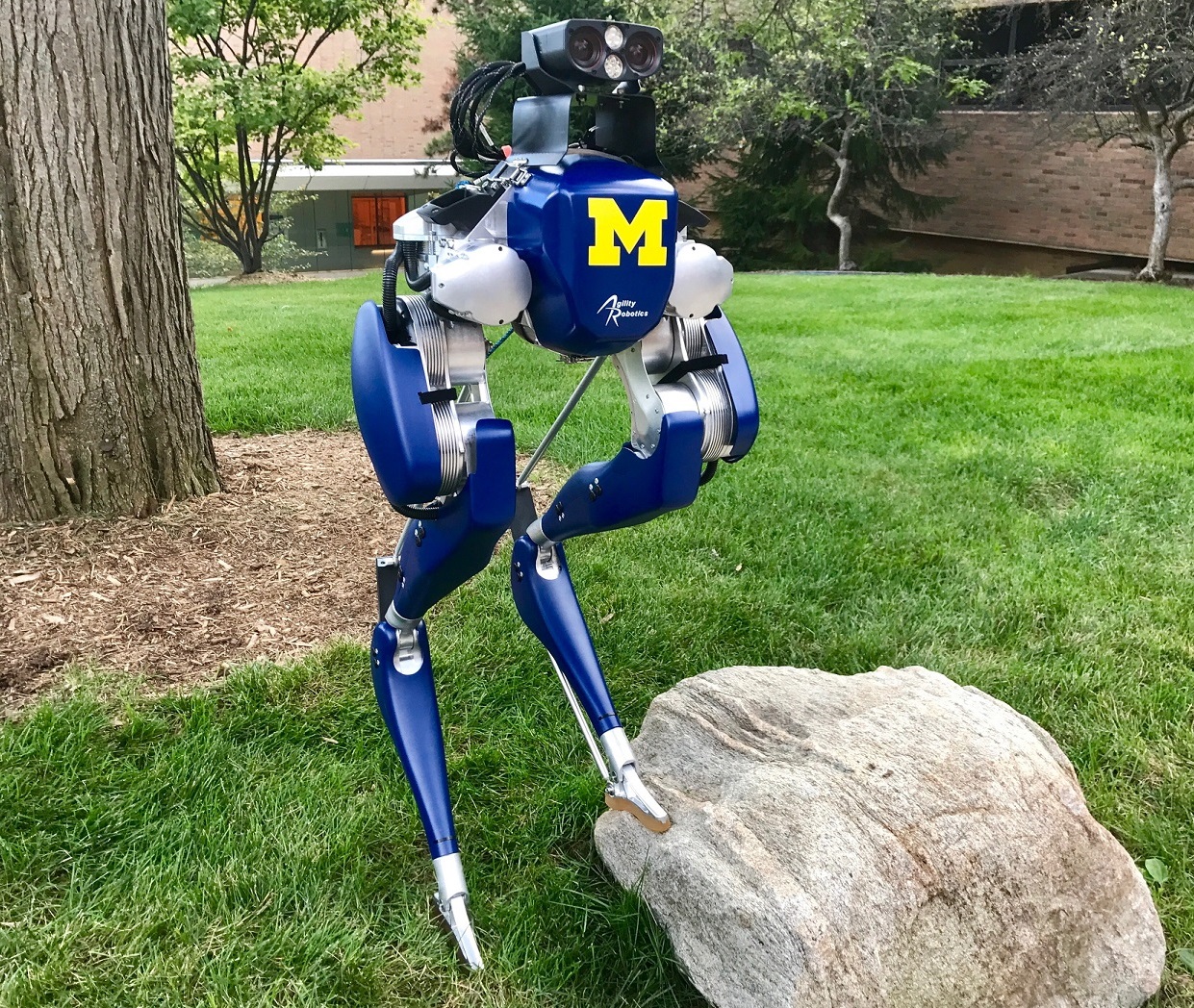
All of these sensors exist on the University of Michigan’s version of the Cassie robot (developed by Agility Robotics), which I’ll use as a concrete example.
Factor Graph Formulation
Let’s see how we can create a factor graph using these 4 sensor types to estimate the trajectory of a legged robot. Each node in the graph represents the robot’s state at a particular timestep. This state includes the 3D orientation, position, and velocity of the robot’s base frame along with the IMU biases. We also include the pose of the contact frame (where the foot hits the ground) to this list of states. For simplicity, the base frame is assumed to be collocated with the inertial/vision sensor frames.
Estimated States:
- Base pose,
X- Base velocity,
V- Contact pose,
C- IMU biases,
b
Each independent sensor measurement will place a measurement factor on the graph’s nodes. Solving the factor graph consists of searching for the maximum a posteriori state estimate that minimizes the error between the predicted and actual measurements.
The robot’s inertial measurements can be incorporated into the graph using the preintegrated IMU factor built into GTSAM 4.0. This factor relates the base pose, velocity, and IMU biases across consecutive timesteps.
Vision data can be incorporated into the graph using a number of different factors depending on the sensor type and application. Here we will simply assume that vision provides a relative pose factor between two nodes in the graph. This can be from either visual odometry or loop closures.
At each timestep, the joint encoder data can be used to compute the relative pose transformation between the robot’s base and contact frames (through forward kinematics). This measurement be captured in a unary forward kinematic factor.
Of course, adding the forward kinematic factor will not affect the optimal state estimate unless additional constraints are placed on the contact frame poses. This is achieved using a binary contact factor which uses contact measurements to infer the movement of the contact frame over time. The simplest case being contact implies zero movement of this frame. In other words, this contact factor tries to keep the contact pose fixed across timesteps where contact was measured. When contact is absent, this factor can simply be omitted in the graph.
If we know how the contact frame moves over time and we can measure the relative pose between the robot’s contact and base frames, then we have an implicit measurement of how the robot’s base moves over time.
The combined forward kinematic and contact factors can be viewed as kinematic odometry measurements of the robot’s base frame.
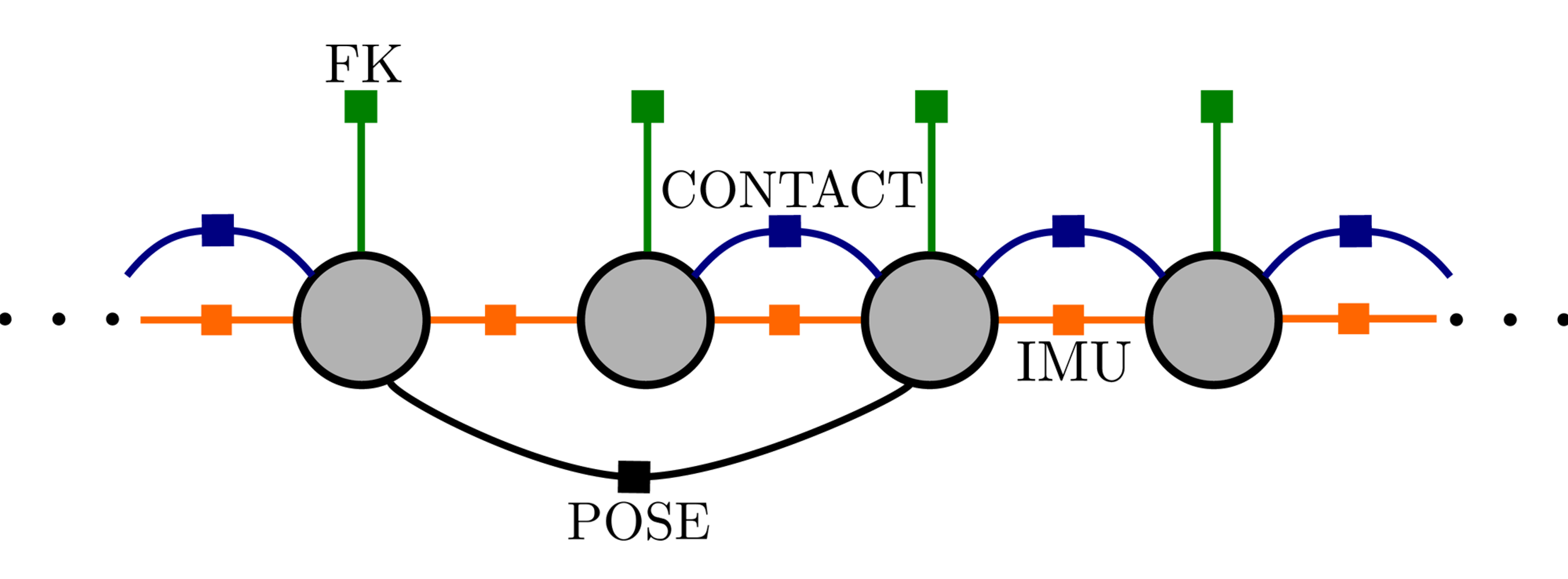
All together, a typical legged robot factor graph may be represented by the picture below. It will contain inertial, vision, forward kinematic, and contact factors.
Forward Kinematic Factor
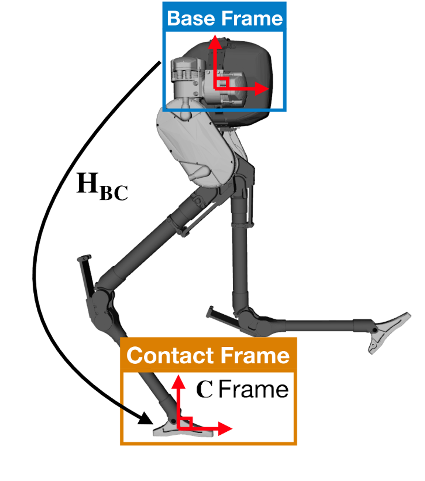
The forward kinematics factor relates the base pose to the current contact pose using noisy encoder measurements. This is a simple relative pose factor which means we can use GTSAM’s built in BetweenFactor<Pose3> factor to implement it. We just need to determine what the factor’s covariance will be.
Assuming the encoder noise is gaussian, we can map the encoder covariance to the contact pose covariance using the body manipulator Jacobian of the forward kinematics function. In general, the manipulator Jacobian maps joint angle rates to end effector twist, so it makes sense that it can be used to approximate the mapping of encoder uncertainty through the non-linearities of the robot’s kinematics.
For example, if H_BC is pose of the contact frame relative to the base frame and J_BC is the corresponding body manipulator Jacobian, the forward kinematic factor can be implemented using the following GTSAM code:
Matrix6 FK_Cov = J_BC * encoder_covariance_matrix * J_BC.transpose();
BetweenFactor<Pose3> forward_kinematics_factor(X(node), C(node), H_BC, noiseModel::Gaussian::Covariance(FK_cov));
Rigid Contact Factor
Contact factors come in a number of different flavors depending on the assumptions we want to make about the contact sensor measurements. However, they will all provide a measurement of contact frame odometry (i.e. how to foot will move over time).
For example, in the simplest case, perhaps measuring contact implies that the entire pose of the foot remains fixed. We can call this rigid contact, and it may be a good assumption for many humanoid robots that have large, flat feet. In contrast, we could alternatively assume a point contact, where the position of the contact frame remains fixed, but the foot is free to rotate.
For now, lets look at how we can implement a rigid contact factor. Again, when contact is measured, we assume there is no relative change in the contact frame pose. In other words, the contact frame velocity is zero. This can be implemented in GTSAM using a BetweenFactor<Pose3> factor, where the measurement is simply the identity element.
BetweenFactor<Pose3> contact_factor(C(node-1), C(node), Pose3::identity(), noiseModel::Gaussian::Covariance(Sigma_ij);
Some potential foot slip can be accommodated through the factor’s covariance, Sigma_ij. If we are highly confident that the foot remained fixed on the ground, this covariance should be small. A large covariance implies less confidence in this assumption.
One idea is simply assuming Gaussian noise on the contact frame velocity. In this case, the factor’s covariance will grow with the length of time between the graph nodes. Another idea is to use contact force information to model the factor’s covariance.
What happens when contact is made/broken?
Using the formulation above, every time contact is made or broken, a new node has to be added to the factor graph. This stems from our contact measurement assumption. When the robot loses contact, we have no way to determine the foot movement using contact sensors alone. Our only choice is to add a new node in the graph and omit the contact factor until contact is regained.
This may not be an issue for some slow walking robots where contact states change infrequently, but what about a running hexapod? In that case, the numerous contact changes will lead to an explosion in the number of nodes (and optimization variables) needed in the graph. This ultimately affects the performance of the state estimator by increasing the time it takes to solve the underlying optimization problem.
Thankfully, there is a way around this problem.
Hybrid Rigid Contact Factor
During many types of walking gaits, when one contact is broken, another is made. For example, with bipedal walking, left stance is followed by right stance, then left, then right, and so on. The order on a hexapod might be more complicated, but one fact remains: there is often (at least) one foot on the ground at all times. We can use this knowledge to improve performance in our factor graph by limiting the insertion rate of new graph nodes.
If we choose two arbitrary times (potentially far apart), any single contact is likely to have been broken at some point between them. However, there may be a chain of contact frames that we can swap through to maintain the notion of contact with the environment. Each consecutive pair of contact frames in this chain are related to each other through forward kinematics.
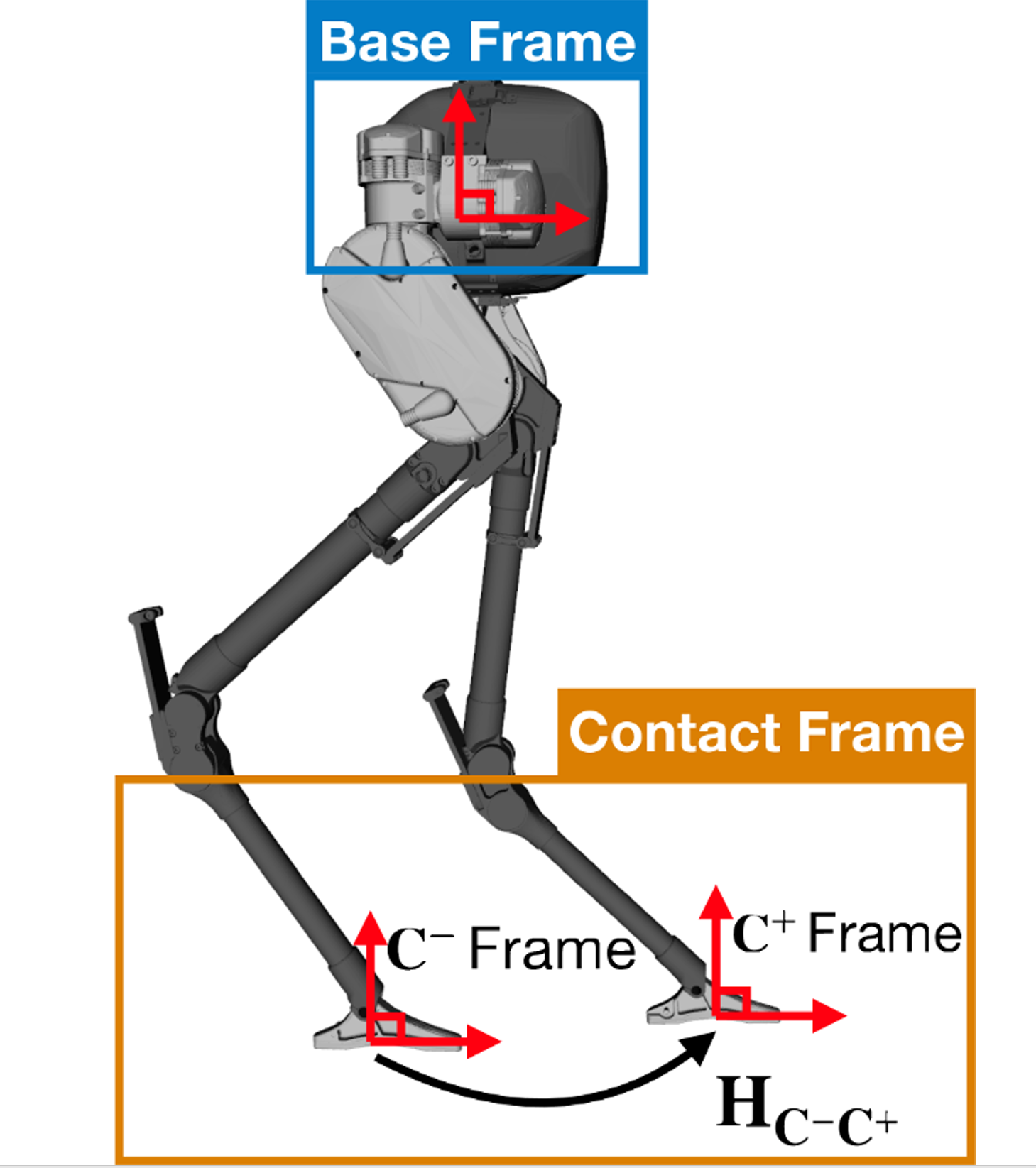
For example, lets say our biped robot switched from left stance (L1), to right stance (R1), back to left stance (L2) again. During the L1 phase, we can assume the contact frame pose remained fixed (zero velocity). When the robot switches from L1 to R1, we can map this contact frame from the left to the right foot using the encoder measurements and forward kinematics (since both feet are on the ground at this time). During the R1 phase, we again assume that the contact pose remains fixed. When the second swap happens, R1 to L2, we map the contact frame back to left foot using the encoder measurements and a (different) forward kinematics function. So in effect, we have tracked the movement of the contact frame across two contact switches. This relative pose measurement provides odometry for the contact frame and can be used to create a hybrid rigid contact factor. Using this method, nodes can now be added to the graph at arbitrary times, and do not have to be added when contact is made/broken (unless all feet come off the ground).
Like the original rigid contact factor, the hybrid version can be created using GTSAM’s BetweenFactor<Pose3> factor, where delta_Hij is the cumulative change in contact pose across all contact switches. The factor’s covariance is typically larger as it needs to account for the uncertainty in each swap’s forward kinematics.
BetweenFactor<Pose3> hybrid_contact_factor(C(node-1), C(node), delta_Hij, noiseModel::Gaussian::Covariance(Sigma_ij);
Coming soon…
I briefly discussed two types of factors that can be used to improve legged robot state estimation: the forward kinematic factor and the (hybrid) rigid contact factor. Combining these two factors allows for kinematic odometry to be added alongside other measurements (inertial, vision, etc.) when building up a factor graph.
In particular, when developing the rigid contact factor, we made the strong assumption that a contact measurement implies zero angular and linear velocity of the contact frame. The factor tries to keep the entire pose of the foot fixed across two timesteps. This assumption may not be valid for all types of walking robots. In fact, it doesn’t even hold for the Cassie robot! The roll angle about Cassie’s foot is unactuated and free to move during walking. In the next post, I will discuss the (hybrid) point contact factor which makes no assumptions about the angular velocity of the contact frame.